Finite difference scheme for multi term variable order fractional diffusion equation

R E S E A R C H

Open Access

Finite difference scheme for multi-term

variable-order fractional diffusion equation

Tao Xu , Shujuan Lü

*

_{, Wenping Chen and Hu Chen}

*_{Correspondence: [email protected]} School of Mathematics and Systems Science, Beihang University, Beijing, P.R. China

Abstract

In this paper, we consider a multi-term variable-order fractional diffusion equation on a finite domain, which involves the Caputo variable-order time fractional derivative of order

α

(x,t)∈(0, 1) and the Riesz variable-order space fractional derivatives of order

β

(x,t)∈(0, 1),

γ

(x,t)∈(1, 2). Approximating the temporal direction derivative by L1-algorithm and the spatial direction derivative by the standard and shifted Grünwald method, respectively, a characteristic finite difference scheme is proposed. The stability and convergence of the difference schemes are analyzed via

mathematical induction. Some numerical experiments are provided to show the efficiency of the proposed difference schemes.

Keywords: Multi-term fractional diffusion equation; Variable-order fractional derivatives; Difference scheme; Stability; Convergence

1 Introduction

As far as we are concerned, the theory of fractional partial differential equations (FPDE), as a new and effective mathematical tool, is very popular and important in many scientific and engineering problems. This is due to the fact that they can well describe the mem-ory and hereditary properties of different substances [1–5]. For instance, the multi-term FPDEs have been employed to some models for describing the processes in practice, such as the oxygen delivery through a capillary to tissues [6], the underlying processes with loss [7], the anomalous diffusion in highly heterogeneous aquifers and complex viscoelas-tic materials [8], and so on. For others, one may refer to [1, 9–13].

Recently, researchers have found that many important dynamic processes exhibit fractional-order behavior that may vary with time and/or space. So it is significant to de-velop the concept of variable-order calculus. Presently, variable-order calculus has been applied in many fields such as viscoelastic mechanics [14], geographic data [15], signal confirmation [16], and diffusion process [17]. Since the kernel of the variable-order oper-ators has a variable exponent, analytical solutions to variable fractional-order differential equations are more difficult to obtain. Therefore, the development of numerical methods to solve variable-order fractional differential equations is an actual and important prob-lem. Nowadays numerical methods for variable-order fractional differential equations, which mainly cover finite difference methods [18–26], spectral methods [27–29], matrix methods [30, 31], reproducing kernel methods [32, 33], and so on, have been studied ex-tensively by many researchers.

Roughly speaking, the fractional models can be classified into three principal kinds: space-fractional differential equation, fractional differential equation, and time-space fractional differential equation. Lately, Shen et al. [18] proposed numerical tech-niques for the variable-order time fractional diffusion equation. Zhang et al. studied an implicit Euler numerical method for the time variable fractional-order mobile-immobile advection-dispersion model in [19]. Lin et al. [20] investigated the stability and conver-gence of an explicit finite-difference approximation for the variable-order nonlinear frac-tional diffusion equation. Zhuang et al. [21] proposed explicit and implicit Euler approx-imations for the variable-order fractional advection-diffusion equation with a nonlinear source term. Sweilam et al. used an explicit finite difference method to study the variable-order nonlinear space fractional wave equation [22]. Zhuang et al. [23] proposed an im-plicit Euler approximation for the time and space variable fractional-order advection-dispersion model with first-order temporal and spatial accuracy.

But in the existing literature, there is little work on higher-order numerical methods for the multi-term time-space variable-order fractional differential equations because more numerical analysis is involved.

In this paper, we consider the following multi-term time-space variable-order fractional diffusion equations with initial-boundary value problem:

⎧

tives defined by [21]

C

Here, left-hand side and right-hand side variable-order Riemann–Liouville fractional derivatives are defined by

Dζ_–(x,t)u(x,t) = proximate the temporal direction derivative, the standard and shifted Grünwald method to approximate the spatial direction derivative, and propose an unconditionally stable fi-nite difference scheme. Furthermore, we prove the convergence of the scheme by using errors estimation method, and the convergence rate of order (τ+h) is obtained.

The remainder of the paper is organized as follows. In Sect. 2, we give some preliminar-ies, which is necessary for our following analysis. A finite difference scheme for equations (1)–(3) is proposed, and the unconditional stability and convergence of the approximation scheme are proved in Sect. 3. Numerical examples are given in Sect. 4 to demonstrate the effectiveness of the scheme. Finally, we conclude this paper in Sect. 5.

2 Preliminaries and discretization of the diffusion equation

Lettk=kτ,k= 0, 1, 2, . . . ,n,xi=ih,i= 0, 1, 2, . . . ,m, whereτ =T/nandh=L/mare time

and space steps, respectively. For an arbitrary function of two variablesu(x,t), we denote

uk_i =u(xi,tk). LetP(x,t) =p(x,t)×(–secβ(x,t)π/2),Q(x,t) =q(x,t)×(–secγ(x,t)π/2).

For a variable-order Caputo derivative, the authors proposed the L1 operator in [19] as follows:

For a variable-order Grünwald–Letnikov fractional derivative, [21, 34] proposed the fol-lowing “standard” and “shifted” operators:

+D

Suppose that the functionf(x) is (m– 1)-continuously differentiable in the interval [0,L] and thatfm_{(x) is integrable in [0,L]. Then, for everyζ(x,t) (0≤m– 1 <ζ(x,t) <m), the}

Define the function space as follows:

and the “shifted” Grünwald approximation

Rζ

It was shown in [34] that whenβ∈(1, 2) using the “standard” Grünwald formula will be unconditionally unstable. So we adopt the “shifted” Grünwald formula to approximate the space fractional derivativesxRβ(x,t)u(x,t) and the “standard” Grünwald formula to

approx-imate the space fractional derivativesxRγ(x,t)u(x,t).

At the end of this section, we give the following discretization schemes for Eq. (1)–(3):

Lα

Fori= 1, 2, . . . ,m– 1,j= 1, 2, . . . ,m– 1,k= 0, 1, 2, . . . ,n,

Therefore, the discrete scheme (4) can be expressed in the following vector form:

⎧ ⎨ ⎩

Ak+1Vk+1=Bk+1, k= 0, 1, . . . ,n– 1,

V0_=φ. (8)

3 Solvability, stability and convergence

In this section, we consider the solvability, stability and convergence of the discrete scheme (4) or (8). For this purpose, we give the following two lemmas.

+

S

s=1

(2 –α₀k_i)

(2 –α_sik)a

k siτ

αk_0i–αk_si

2(k–j+ 1)1–αsik_{– (k–j)}1–αksi_{– (k–j+ 2)}1–αksi ≥0.

In addition, noting that (Mk

i,0)–1Mki,0= 1, we can obtain the second formula of the lemma.

The proof is completed.

Lemma 3.2([23]) For1 <β≤β(x,t)≤β< 2, 0 <γ ≤γ(x,t)≤γ < 1,the coefficients gj

β_ik

and gj

γ_ik(i= 1, 2, . . . ,m,k= 1, 2, . . . ,n)satisfy

g0

β_ik= 1; g

1

βk_i < 0; g

j

β_ik> 0, (j≥2);

∞

j=0

gj

βk_i = 0;

l

j=0

gj

β_ik< 0, (l≥1).

g_γ0k

i = 1; g j

γ_ik< 0, (j≥1);

∞

j=0

g_γjk i

= 0;

l

j=0

g_γjk i

> 0, (l≥1).

3.1 Solvability analysis

Using Lemma 3.2 and a simple computation yields

Ak_ii≥1, Ak_ij≤0, (j=i),

m–1

j=1

Ak_ij≥1, i= 1, . . . ,m– 1,

Ak_ii–

m–1

j=1

Ak_ij=Ak_ii+

m–1

j=1

Ak_ij≥1, i= 1, . . . ,m– 1.

(9)

Namely, matrixAis strictly diagonally dominant with positive diagonal terms and non-positive off-diagonal terms. Therefore, matrixAis invertible. So the following theorem can be obtained.

Theorem 3.1 Scheme(8)has a unique solution.

3.2 Stability analysis Theorem 3.2 Suppose Vk

i,Vikare solutions of schemes(4)with the initial values V0k,V0k,

respectively.Then

_Vk_–Vk

∞≤CV0–V0∞, k= 0, 1, . . . ,

whereVk_–Vk_∞=max

1≤i≤m–1|vki –vki|.

Proof DenoteXk_=Vk_–Vk_{= (ε}k

1, . . . ,εmk–1)T, then

Ak+1Xk+1=Bk+1, k= 0, 1, . . . ,n– 1, (10)

where the component ofBk+1_is

Bk_i+1=M_ik_,0+1 –1

k

j=1

Now we prove this theorem applying mathematical induction method.

Fork= 1, supposeX1∞=|ε1_l|. Considering thelth equation of (10), we have

A1_llε1_l=

B1l –

m–1

j=1,j=l

A1_ljε1_j

≤B1l+ m–1

j=1,j=l

A1_ljε1_l,

namely

A1_ll–

m–1

j=1,j=l A1_lj

ε1_l≤B1_l.

Due to (9) and (11), we can obtain

ε1_l≤ |B

1 l| |A1

ll|– m–1

j=1,j=l|A1lj|

≤B1_l=ε_l0≤X0_∞.

Assume thatXj_{∞≤ X}0_{∞(j= 1, . . . ,k), similar to the case ofk= 1. SupposeX}k+1_∞= |ε_lk+1|, according to (9), (11), and Lemma 3.1, we have

εk_l+1≤Bk_l+1

=Mk_l,0+1 –1

k

j=1

Mk_l,+1_k–j–M_lk_,+1_k–j+1 ε_lj+Mk_l,0+1 –1Mk_l,+1_k ε0_l

≤Mk_l,0+1 –1

k

j=1

M_lk_,+1_k–j–M_lk_,+1_k–j+1 X0_∞+Mk_l,0+1 –1M_lk_,+1_k X0_∞

≤X0_∞.

Due to the principle of mathematical induction, the proof is completed.

3.3 Convergence analysis

Theorem 3.3 Suppose that problem(1)has a smooth solution u(x,t).Let vk_i be the numer-ical solution computed by(4).Then there is a positive constant C independent ofτ and h such that

uk_i –vk_i∞≤C(τ+h), i= 1, 2, . . . ,m– 1;k= 1, 2, . . . ,n.

Proof DenoteYk_=Uk_–Vk_{= (η}k

1, . . . ,ηmk–1)T, then according to (1) and (4), we obtain the

following error equation:

Lα

k+1 0i

τ ηki+1+ S

s=1

ak+1 si L

α_sik+1

τ ηki+1–Pik+1

ρ_–Dβ

k+1 i h ηk

+1 i +σ+D

β_ik+1

h ηk +1 i

–Qk_i+1ρ_–Dγ

k+1 i h η

k+1 i +σ+D

γ_ik

h η k+1

where

We rewrite it in the following vector form:

Ak+1Yk+1=Bk+1, k= 0, 1, . . . ,n– 1, (12)

where the component ofBk+1is

Bk+1

similar to the proof of Theorem 3.3.

Fork= 1, supposeY1∞=|η_l1|. From Lemma 2.1, Lemma 2.2, the definitions ofMk_i,j,bk_i

Substituting the above inequality into (14), we have

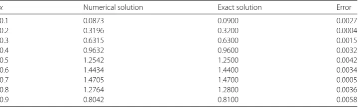
Table 1 Numerical solution, exact solution, and absolute error atT= 1.0 of (15)

x Numerical solution Exact solution Error

0.1 0.0873 0.0900 0.0027

0.2 0.3196 0.3200 0.0004

0.3 0.6315 0.6300 0.0015

0.4 0.9632 0.9600 0.0032

0.5 1.2542 1.2500 0.0042

0.6 1.4434 1.4400 0.0034

0.7 1.4705 1.4700 0.0005

0.8 1.2764 1.2800 0.0036

0.9 0.8042 0.8100 0.0058

Due to the principle of mathematical induction, the theorem is proved.

4 Numerical examples

In this section, three examples are presented to illustrate the practical application of our numerical method. Consider the vectorsVk_{= (v}k

0, . . . ,vkm), where vki is the approximate

solution forxi=ih,i= 0, 1, . . . ,m, at a certain timet, andUk= (uk0, . . . ,ukm), whereuki is the

exact solution. The error is defined by thel∞norms:

Vk–Uk_∞= max

0≤i≤m

vk_i –uk_i.

Example4.1 Consider the following fractional differential equation:

⎧ ⎪ ⎪ ⎪ ⎪ ⎪ ⎨ ⎪ ⎪ ⎪ ⎪ ⎪ ⎩ C

0D

α(x,t)

t u(x,t) + 2cos(β(x,t)π/2)xRβ(x,t)u(x,t) –cos(γ(x,t)π/2)xRγ(x,t)u(x,t)

=f(x,t), (x,t)∈= (0, 1)×(0,T],

u(x, 0) = 5x2_{(1 –x), 0≤x≤1,}

u(0,t) = 0, u(1,t) = 0, 0≤t≤T,

(15)

where

f(x,t) = 10x

2_{(1 –x)t}2–α(x,t)

(3 –α(x,t)) – 10

t2+ 1 2x

2–β(x,t)

(3 –β(x,t))–

6x3–β(x,t)

(4 –β(x,t))

+ 5t2+ 1 2x

2–γ(x,t)

(3 –γ(x,t))–

6x3–γ(x,t)

(4 –γ(x,t))

.

We takeα(x,t) = 0.8 + 0.01sin(5xt),β(x,t) = 1.8 + 0.01x2_t2_{,γ(x,t) = 0.8 + 0.01x}2_sint,ρ=

1,σ= 0,τ=h= 0.1. The above problem has the exact solutionu(x,t) = 5(t2_{+ 1)x}2_{(1 –x).}

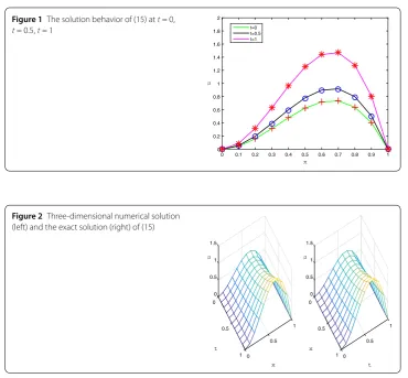
Figure 1The solution behavior of (15) att= 0, t= 0.5,t= 1

Figure 2Three-dimensional numerical solution (left) and the exact solution (right) of (15)

Example4.2 Consider the following fractional differential equation:

⎧ ⎪ ⎪ ⎪ ⎪ ⎪ ⎨ ⎪ ⎪ ⎪ ⎪ ⎪ ⎩ C

0D

α(x,t)

t u(x,t) +cos(β(x,t)π/2)xRβ(x,t)u(x,t) +∂u(x,t)/∂x

=f(x,t), (x,t)∈= (0, 8)×(0,T],

u(x, 0) =x2(8–₈₀x), 0≤x≤8,

u(0,t) = 0, u(8,t) = 0, 0≤t≤T,

(16)

where

f(x,t) = x

2_{(8 –x)t}1–α(x,t)

80(2 –α(x,t))– (t+ 1)

80

16x2–β(x,t)

(3 –β(x,t))–

6x3–β(x,t)

(4 –β(x,t))

+(t+ 1)

80 x(16 – 3x).

We takeα(x,t) = 0.5 + 0.01sin(5xt),β(x,t) = 1.5 + 0.01x2_t2_{,γ(x,t) = 1,ρ= 1,σ= 0,τ =}

0.05,h= 0.1. The above problem has the exact solutionu(x,t) =(t+1)x₈₀2(8–x).

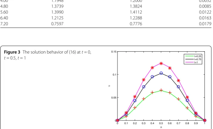
Table 2 Numerical solution, exact solution, and absolute error atT= 1.0 of (16)

x Numerical solution Exact solution Error

0.80 0.0917 0.0864 0.0053

1.60 0.3107 0.3072 0.0035

2.40 0.6056 0.6048 0.0008

3.20 0.9194 0.9216 0.0022

4.00 1.1948 1.2000 0.0052

4.80 1.3739 1.3824 0.0085

5.60 1.3990 1.4112 0.0122

6.40 1.2125 1.2288 0.0163

7.20 0.7597 0.7776 0.0179

Figure 3The solution behavior of (16) att= 0, t= 0.5,t= 1

Example4.3 Consider the two-term VO fractional differential equation:

⎧ ⎪ ⎪ ⎪ ⎪ ⎪ ⎨ ⎪ ⎪ ⎪ ⎪ ⎪ ⎩ C

0D

α(x,t)

t u(x,t) +C0D

α(x,t)/2

t u(t) –xRβ(x,t)u(x,t) +u(x,t) =f(x,t),

(x,t)∈= (0, 1)×(0,T],

u(x, 0) =x2_{(1 –x)}2_{, 0≤x≤1,}

u(0,t) = 0, u(1,t) = 0, 0≤t≤T,

(17)

where

f(x,t) = 2x2(1 –x)2

t2–α(x,t)

(3 –α(x,t))+

t2–α(x,t)/2

(3 –α(x,t)/2)

+sec(β(x,t)π/2) 2

1 +t2

×

2(x2–β(x,t)_{+ (1 –x)}2–β(x,t)₎

(3 –β(x,t)) –

12(x3–β(x,t)_{+ (1 –x)}3–β(x,t)₎

(4 –β(x,t))

+24(x

4–β(x,t)_{+ (1 –x)}4–β(x,t)₎

(5 –β(x,t))

+1 +t2 x2(1 –x)2.

We take α(x,t) = 1 – 0.5e–xt_{,β(x,t) = 1.7 + 0.1e}–₁₀₀₀x2 –₅₀t–1_{, ρ=σ =}1

2,τ =h= 0.1. The

above problem has the exact solutionu(x,t) = (1 +t2)x2(1 –x)2.

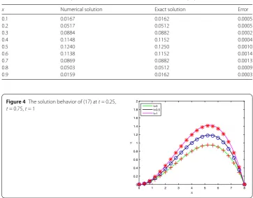
Table 3 Numerical solution,exact solution and absolute error atT= 1.0 of (17)

x Numerical solution Exact solution Error

0.1 0.0167 0.0162 0.0005

0.2 0.0517 0.0512 0.0005

0.3 0.0884 0.0882 0.0002

0.4 0.1148 0.1152 0.0004

0.5 0.1240 0.1250 0.0010

0.6 0.1138 0.1152 0.0014

0.7 0.0869 0.0882 0.0013

0.8 0.0503 0.0512 0.0009

0.9 0.0159 0.0162 0.0003

Figure 4The solution behavior of (17) att= 0.25, t= 0.75,t= 1

5 Conclusion

In this paper, a finite difference scheme has been proposed to solve a multi-term time-space variable-order fractional diffusion equation. The stability and convergence have been analyzed by the mathematical induction method. Numerical examples are provided to show that the finite difference scheme is computationally efficient. The techniques for the numerical schemes and related numerical analysis can be applied to solve variable-order fractional (in space and/or in time) partial differential equations.

Acknowledgements

The work was supported by the National Natural Science Foundation of China (No. 11672011, 11272024 ).

Competing interests

The authors declare that they have no competing interests.

Authors’ contributions

TX wrote the first draft and SL corrected and improved the final version. Both authors read and approved the final draft.

Publisher’s Note

Springer Nature remains neutral with regard to jurisdictional claims in published maps and institutional affiliations.

Received: 9 November 2017 Accepted: 5 March 2018 References

1. Podlubny, I.: Fractional Differential Equations. Academic Press, San Diego (1999)

2. Trujillo, J.J., Kilbas, A.A., Srivastava, H.M.: Theory and Applications of Fractional Differential Equations. Elsevier, Amsterdam (2006)

3. Ross, B., Miller, K.S.: An Introduction to the Fractional Calculus and Fractional Differential Equations. Wiley, New York (1993)

4. Meerchaert, M.M., Benson, D.A., Wheatcraft, S.W.: Application of a fractional advection-dispersion equation. Water Resour. Res.36, 1403–1412 (2000)

6. Srivastava, V., Rai, K.N.: A multi-term fractional diffusion equation for oxygen delivery through a capillary to tissues. Math. Comput. Model.51, 616–624 (2010)

7. Luchko, Y.: Initial-boundary-value problems for the generalized multi-term time-fractional diffusion equation. J. Math. Anal. Appl.374, 538–548 (2011)

8. Liu, Y., Zhou, Z., Jin, B., Lazarov, R.: The Galerkin finite element method for a multi-term time-fractional diffusion equation. J. Comput. Phys.281, 825–843 (2015)

9. McGough, R., Zhuang, P., Liu, Q., Liu, F., Meerschaert, M.M.: Numerical methods for solving the multi-term time fractional wave equations. Fract. Calc. Appl. Anal.16, 9–25 (2013)

10. Anh, I., Turner, I., Ye, H., Liu, F.: Maximum principle and numerical method for the multi-term time-space Riesz–Caputo fracional differential equations. Appl. Math. Comput.227, 531–540 (2014)

11. Bai, Y.R., Liu, Z.H., Zeng, S.D.: Maximum principles for multi-term space-time variable-order fractional diffusion equation and their applications. Fract. Calc. Appl. Anal.19, 188–211 (2016)

12. Jia, X.Z., Du, D.H., Li, G.S., Sun, C.L.: Numerical solution to the multi-term time fractional diffusion equation in a finite domain. Numer. Math., Theory Methods Appl.9, 337–357 (2016)

13. Sun, Z.Z., Gao, G.H., Alikhanov, A.A.: The temporal second order difference schemes based on the interpolation approximation for sloving the time multi-term and distributed-order fractional sub-diffusion equations. J. Sci. Comput.73, 93–121 (2017)

14. Coimbra, C.F.M.: Mechanica with variable-order differential operators. Ann. Phys.12, 692–703 (2003)

15. Cowan, D.R., Cooper, G.R.J.: Filtering using variable order vertical derivatives. Comput. Geosci.30, 455–459 (2004) 16. Tseng, C.C.: Design of variable and adaptive fractional order fir differentiators. Signal Process.86, 2554–2566 (2006) 17. Chen, Y., Sun, H., Chen, W.: Variable-order fractional differential operators in anomalous diffusion modeling. Physica A

388, 4586–4592 (2009)

18. Chen, J., Turner, I., Anh, V., Shen, S., Liu, F.: Numerical techniques for the variable order time fractional diffusion equation. Appl. Math. Comput.218, 10861–10870 (2012)

19. Phanikumar, M.S., Meerschaert, M.M., Zhang, H., Liu, F.: A novel numerical method for the time variable fractional order mobile-immobile advection-dispersion model. Comput. Math. Appl.66, 693–701 (2013)

20. Anh, V., Lin, R., Liu, F., Turner, I.: Stability and convergence of a new explicit finitedifference approximation for the variable-order nonlinear fractional diffusion equation. Appl. Math. Comput.212, 435–445 (2009)

21. Ahn, V., Turner, I., Zhuang, P., Liu, F.: Numerical methods for the variable-order fractional advection-diffusion equation with a nonlinear source term. SIAM J. Numer. Anal.47, 1760–1781 (2009)

22. Almarwm, H.M., Sweilam, N.H., Khader, M.M.: Numerical studies for the variable-order nonlinear fractional wave equation. Fract. Calc. Appl. Anal.15, 669–683 (2012)

23. Zhuang, P., Turner, I., Anh, V., Zhang, H., Liu, F.: Numerical analysis of a new space-time variable fractional order advection-dispersion equation. Appl. Math. Comput.242, 541–550 (2014)

24. Anh, V., Turner, I., Chen, C.M., Liu, F.: Numerical schemes with high spatial accuracy for a variable-order anomalous subdiffusion equation. SIAM J. Sci. Comput.32, 1740–1760 (2010)

25. Qiu, Y.N., Cao, J.X.: A compact finite difference scheme for variable order subdiffusion equation. Commun. Nonlinear Sci. Numer. Simul.48, 140–149 (2017)

26. Karniadakis, G.E., Zhao, X., Sun, Z.Z.: Second-order approximations for variable order fractional derivatives: algorithms and applications. J. Comput. Phys.293, 184–200 (2015)

27. Zaky, M.A., Bhrawy, A.H.: Numerical algorithm for the variable-order Caputo-fractional functional differential equation. Nonlinear Dyn.85, 1818–1823 (2016)

28. Karniadakis, G.E., Zayernouri, M.: Fractional spectral collocation methods for linear and nonlinear variable order fpdes. J. Comput. Phys.293, 312–338 (2015)

29. Zakyb, M.A., Bhrawya, A.H.: Highly accurate numerical schemes for multi-dimensional space variable-order fractional Schrödinger equations. Comput. Math. Appl.73, 1100–1117 (2017)

30. Chen, Y.M., Wei, Y.Q., Liu, D.Y., Yu, H.: Numerical solution for a class of nonlinear variable order fractional differential equations with Legendre wavelets. Appl. Math. Lett.46, 83–88 (2015)

31. Li, B.F., Sun, Y.N., Chen, Y.M., Li, L.Q.: Numerical solution for the variable order linear cable equation with Bernstein polynomials. Appl. Math. Comput.238, 329–341 (2014)

32. Wu, B.Y., Li, X.Y.: A numerical technique for variable fractional functional boundary value problems. Appl. Math. Lett.

43, 108–113 (2015)

33. Wu, B.Y., Li, X.Y.: A new reproducing kernel method for variable order fractional boundary value problems for functional differential equations. J. Comput. Appl. Math.311, 387–393 (2017)

34. Tadjeran, C., Meerschaert, M.M.: Finite difference approximations for fractional advection-dispersion flow equations. J. Comput. Appl. Math.172, 65–77 (2004)