R E S E A R C H
Open Access
A parameter uniform difference scheme
for the parameterized singularly perturbed
problem with integral boundary condition
Mustafa Kudu
1**Correspondence:
1Department of Mathematics,
Faculty of Arts and Sciences, Erzincan University, Erzincan, Turkey
Abstract
We consider a uniform finite difference method on a Bakhvalov mesh to solve a quasilinear first order parameterized singularly perturbed problem with integral boundary conditions. Uniform first order error estimates in the discrete maximum norm have been established. Numerical results that demonstrate the sharpness of our theoretical analysis are presented.
MSC: 65L11; 65L12; 65L20
Keywords: Singular perturbation; Finite difference scheme; Uniform convergence; Parameterized problem; Bakhvalov mesh; Integral boundary condition
1 Introduction
Singularly perturbed differential equations are typically characterized by a small parame-terεmultiplying some or all of the highest order terms in the differential equations as nor-mally boundary layers occur in their solutions. These equations play an important role in today’s advanced scientific computations. Many mathematical models starting from fluid dynamics to the problems in mathematical biology are modeled by singularly perturbed problems. Typical examples include high Reynold’s number flow in the fluid dynamics, heat transport problem, etc. For more details on singular perturbation, one can refer to the books [1–4] and the references therein. The numerical analysis of singular perturba-tion cases has always been far from trivial because of the boundary layer behavior of the solution. Such a problem undergoes rapid changes within very thin layers near the bound-ary or inside the problem domain [2, 3]. It is well known that standard numerical methods for solving such problems are unstable and fail to give accurate results when the perturba-tion parameter is small. Therefore, it is important to develop suitable numerical methods to the problems, whose accuracies do not depend on the parameter value, i.e., methods that are convergentε-uniformly. For the various approaches on the numerical solutions of differential equations with steep, continuous solutions, we may refer to the monographs [1, 4, 5].
In this paper, we consider the following parameterized singular perturbation problem with integral boundary condition arising in many scientific applications [6, 7] (see also
references therein):
εu+f(t,u,λ) = 0, t∈= (0,T),T> 0, (1) u(0) +
T
0
c(s)u(s)ds=A, (2)
u(T) =B, (3)
whereε∈(0, 1] is the perturbation parameter,λis known as the control parameter,Aand Bare given constants. The functionsc(t)≥0 andf(t,u,λ) are assumed to be sufficiently continuously differentiable for our purpose in=∪ {t= 0}and×R2, respectively, and moreover
0 <α≤∂f ∂u ≤a
∗<∞,
0 <m1≤ ∂f
∂λ
≤M1<∞.
By a solution of (1)–(3) we mean{u(t),λ} ∈C1[0,T]×R, for which problem (1)–(3) is
satisfied. Under these assumptions, problem (1)–(3) has a unique solutionu(t). Forε 1, the functionu(t) has in general a boundary layer of widthO(ε) neart= 0 (see [8–10]).
Parameterized boundary value problems have been considered by many researchers for many years. Such problems arise in physical chemistry and physics, describing the exothermic and isothermal chemical reactions, the steady-state temperature distribu-tions, the oscillation of a mass attached by two springs leading to a differential equation with a parameter [5, 11, 12]. An overview of some existence and uniqueness results and ap-plications of parameterized equations may be obtained, for example, in [11–14](see also references therein). In [11, 12, 14, 15], the authors have also considered some approxi-mating aspects of this kind of problems. But in the above-mentioned papers, algorithms are only concerned with the regular cases (i.e., when the boundary layers are absent). In recent years, many researchers presented the numerical methods for the singular pertur-bation cases of parameterized problems. Uniform convergent finite-difference schemes for solving parameterized singularly perturbed two-point boundary value problems have been considered in [8, 10, 15–22] (see also references therein). In [8, 10, 16, 17, 19, 20] authors used the boundary layer technique for solving an analogous problem. A method-ology based on the homotopy analysis technique to approximate the analytic solution was investigated in [15, 21, 22].
second order convergent on Shishkin mesh, was discussed in [30] (see also [20, 33]). For the numerical methods concerning second order singularly perturbed differential equa-tions with integral boundary condiequa-tions, one can see, e.g., [28, 29, 31].
In this paper, as far as we know, the numerical solution of the singularly perturbed boundary value problem containing both control parameter and integral condition is first being considered. For the numerical solution of such problems, a specific approach is re-quired to construct the appropriate difference scheme and examining the error analysis. The scheme is constructed by the method of integral identities with the use of appropri-ate quadrature rules with the remainder terms in integral form. The aim here is to con-struct anε-uniformly numerical method which givesε-uniformly convergent numerical approximations to solve problem (1)–(3). For this, we use a finite difference scheme on a Bakhvalov mesh which is dense in the initial layer. The Bakhvalov mesh is dependent on
εand mesh points have to be condensed in a neighborhood oft= 0 in order to resolve the initial layer. In the Bakhvalov mesh, basically half of the mesh points are concentrated in O(ε|lnε|) neighborhood of the pointt= 0 and the remaining half forms a uniform mesh on the rest of [0,T] (see [2, 4, 10, 30, 32, 34, 35]). We show that the proposed scheme is uniformly convergent in the discrete maximum norm accuracy ofO(N–1) on Bakhvalov meshes. Note that, in [10], the first order convergent difference scheme in Bakhvalov type mesh under the first type boundary conditions for equation (1.1) was presented. Also, in the above-mentioned work [9] that includes integral boundary condition, while condi-tions (2.1) and (4.8) are generally provided for sufficiently small values ofε, as the integral boundary condition of our work is more general, and the convergence is uniform for both small and moderate values of perturbation parameterε.
The paper is organized as follows. In Sect. 2, the difference scheme constructed on the non-uniform mesh for the numerical solution (1)–(3) is presented and graded mesh is introduced. The uniform convergence of the difference scheme is investigated and error of the difference scheme is evaluated in Sect. 3. Finally, in Sect. 4 some numerical results are presented to confirm the theoretical analysis. The paper ends with conclusions.
Henceforth,Candcdenote the generic positive constants independent of both the per-turbation parameterεand the mesh parameterN. Such a subscripted constant is fixed. We also will useg∞=max0≤t≤T|g(t)|for anyg∈C[0,T].
2 The finite difference scheme
To construct the numerical method and for convergence analysis, we need the asymptotic estimates for the differential solution{u(t),λ}.
Lemma 2.1 The solution{u(t),λ}of problem(1)–(3)satisfies the following bounds:
|λ| ≤c0, (4)
u∞≤c1, (5)
where
c0=m–11
α|A| eαT– 1+
|B|a∗(1 –c∞T) m1(ea∗T– 1)
+F∞
,
c1=A+α–1
1 +c∞TF∞+M1c0
and
u(t)≤C
1 +1
εe
–αtε , t∈[0,T], (6)
provided a∈C1[0,T]and|∂f
∂t| ≤C for t∈[0,T].
Proof One can prove this result following the method given in [9], Lemma 2.1, and in [10],
Lemma 2.1.
LetωN be any non-uniform mesh on:
ωN={0 <t1<t2<· · ·<tN–1<tN=T}
andω¯N =ωN ∪ {t= 0}. For eachi≥1, we set the step sizehi=ti–ti–1. To simplify the
notation, we setgi=g(ti) for any functiong(t), whilegiN denotes an approximation ofg(t) atti. For any mesh function{wi}defined onωN, we use
wt,i= (wi–wi–1)/hi,
w∞≡ w∞,ω¯N:= max
0≤i≤N|wi|.
To obtain approximation for (1), we integrate (1) over (ti–1,ti):
εut,i+h–1i
ti
ti–1
ft,u(t),λdt= 0, 1≤i≤N,
which yields the relation
εut,i+f(ti,ui,λ) +Ri= 0, 1≤i≤N, (7)
with local truncation error
Ri= –h–1i
ti
ti–1
(t–ti–1)
d dtf
t,u(t),λdt. (8)
To define an approximation for the boundary condition (2), here we use the composite right-hand side rectangle rule:
u(0) +
T
0
c(s)u(s)ds=u0+
N
i=1
hiciui+r
with remainder term
r= – N
i=1 ti
ti–1
(t–ti–1)
d dt
Consequently,
u0+
N
i=1
hiciui+r=A. (10)
NeglectingRiandrin (7) and (10), we propose the following difference scheme for ap-proximating (1)–(3):
εuN¯t,i+fti,uNi ,λN
= 0, 1≤i≤N, (11)
uN0 + N
i=1
hiciuNi =A, (12)
uN
N =B. (13)
For the difference scheme (11)–(13) to beε-uniformly convergent, we will use the B-mesh. For an even numberN, the B-mesh takesN/2 + 1 points in the interval [0,σ] and also N/2 + 1 points in the interval [σ,T], where the transition pointσ, which separates the fine and coarse portions of the mesh, is obtained by taking
σ=min
T 2,α
–1ε|lnε|
. (14)
In practice one usually hasσ T, so the mesh is fine on [0,σ] and coarse on [σ,T]. We shall consider a meshωNwhich is equidistant in [σ,T] but graded in [0,σ] by a logarithmic mesh generating function. The corresponding mesh points are
ti∈[0,σ] :ti=
⎧ ⎨ ⎩
–α–1εln[1 – (1 –ε)2i
N], ifσ<T/2,
–α–1εln[1 – (1 –exp(–α2Tε))N2i], ifσ=T/2,i= 0, . . . ,N/2,
(15)
ti∈[σ,T] :ti=σ+ (i–N/2)h, i=N/2 + 1, . . . ,N,h= 2(T–σ)/N. (16) In the rest of the paper we only consider B-mesh defined by (14)–(16).
3 Uniform convergence and error estimates
To investigate the convergence of the method, note that the error functionszNi =uNi –ui, 0≤i≤N,μN =λN–λare the solution of the discrete problem
εzN¯t,i+fti,uNi ,λN
–f(ti,ui,λ) =Ri, 1≤i≤N, (17)
z0N+ N
i=1
hicizNi –r= 0, (18)
zNN= 0, (19)
where the truncation errorsRiandrare given by (8) and (9), respectively.
Before estimating errors of the approximate solution, we need the known equalities for the first order difference equation, namely, the solution of
can be expressed in the following forms:
yi=y0Qi+ i
k=1
ϕkQi–k (20)
or
yi=yNQ–1N–i– N
k=i+1
ϕkQ–1k–i, (21)
where
Qi–k=
⎧ ⎨ ⎩
1, k=i,
i
=k+1q, 1≤k≤i– 1.
Relations (20) and (21) can be easily verified by induction ini.
Lemma 3.1 For the solution of(17)–(19),the following estimates hold:
μN≤C|r|, (22)
zN0≤ |r|+c∞TBNμNM1+R∞, (23)
zNi ≤z0N+α–1M1μN+R∞
, 1≤i≤N– 1, (24)
where
BN= N
=1
h
ε+ah
QN–,
QN–= ⎧ ⎨ ⎩
1, for=N,
N s=+1
ε
ε+ashs, for1≤≤N– 1. Proof Equation (17) can be rewritten as
εzN¯t,i+aiziN=biμN+Ri, 1≤i≤N– 1, (25)
with
ai=
∂f
∂u
ti,ui+γzNi ,λ+γ μN
,
bi= –
∂f
∂λ
ti,ui+γzNi ,λ+γ μN
, 0 <γ < 1.
From (25) we have
zN i =
ε ε+aihi
zN i–1+μN
hibi
ε+aihi
+ hiRi
Solving the first-order difference equation with respect tozNi by using (21) and setting the boundary condition (19), we get
ziN= –μN
Taking into consideration in (26) the integral boundary condition (18), we have
μN =N r
Now, we estimate separately the terms on the right-hand side of equality (27). For the first term, we have
After taking into consideration (28) and (29) in (27), we arrive at (22). Now, we need to estimatez0. From (26), by using (20) we have
From here, by virtue of (18) it follows that
≤ |r|+c∞TM1μN+R∞ N
=1
h
ε+ah
QN–,
which implies validity of (23).
Finally, applying the maximum principle for the difference operatorLNzN
i :=εzN¯t,i+aiz N i , 1≤i≤N, to Eq. (25) immediately leads to (24).
Lemma 3.2 The error functions R and r satisfy
R∞,ωN ≤CN
–1, (30)
|r| ≤CN–1. (31)
Proof We first give proof for (30). From explicit expression (8) forRi, on an arbitrary mesh we have
|Ri| ≤h–1i
ti
ti–1
(t–ti–1) ∂f
∂t
t,u(t),λ+∂f
∂u
t,u(t),λu(t)dt
≤Ch–1i
ti
ti–1 (t–ti–1)
1 +u(t)dt, 1≤i≤N.
This inequality together with (6) enables us to write
|Ri| ≤C
h–1i +h–1i ε–1
ti
ti–1
(t–ti–1)e–αt/εdt
, 1≤i≤N. (32)
Riis estimated on [0,σ] and [σ,T] separately. We consider first the caseα–1ε|lnε|<T/2, and soσ=α–1ε|lnε|. In [σ,T], which is outside the layer|u(t)| ≤C(orε–1e–αx/ε≤1) by
(6) andhi=h. Hereby, from (32) we get
|Ri| ≤2C(T–σ)N–1, i=N/2 + 1, . . . ,N. (33)
On the other hand, in the layer region [0,σ], by (6), inequality (32) becomes
|Ri| ≤C
hi+α–1
e–αtiε–1 +e– αti
ε , i= 1, . . . ,N/2. (34)
Since
hi=ti–ti–1=α–1ε
–ln
1 – (1 –ε)2i N
+ln
1 – (1 –ε)2(i– 1) N
≤2α–1(1 –ε)N–1
and
e–αtiε–1 +e– αti
ε = 2(1 –ε)N–1, it then follows from (34) that
Now consider the caseσ=T/2 and soσ=α–1ε|lnε|. Therefore, fort
it follows from (32) that
|Ri| ≤C
T+ 2 eα N
–1, i=N/2 + 1, . . . ,N, (36)
and this together with (36) gives the bound
|Ri| ≤CN–1.
Inequalities (33), (35), and (36) finish the proof of (30).
Finally, we estimate the remainder termr. From the explicit expression (9) we obtain
|r| ≤
This inequality together with (6) reduces to
|r| ≤ c∞C
From (37), the validity of (31) follows:
|r| ≤C
ωN,respectively.Then the following estimates hold:
λ–λN≤CN–1,
u–uN∞, N ≤CN
–1.
4 Algorithm and numerical results
The results of the numerical experiment are presented in this section, which confirms the theoretical bounds established in the previous section.
(a) We solve the nonlinear problem (11)–(13) using the following quasilinearization technique:
λ(n)=λ(n–1)–(B–u
(n–1)
N–1)ρN–1+f(T,B,λ(n–1))
∂f/∂λ(T,B,λ(n–1)) ,
u(0n)=A–cNhNB– N–1
i=1
hibiu(in–1),
u(in)=u(in–1)–(u
(n–1)
i –u
(n)
i–1)ρi–1+f(ti,u(in–1),λ(n))
∂f/∂u(ti,ui(n–1),λ(n)) +ρi–1
, n= 1, 2, . . . ,
whereρi=hi/ε;λ(0)andu(0)i (1≤i≤N– 1) are the initial iterations given. (b) Consider the test problem:
εu+ 2u–e–u+t2+λ+tanh(λ+t) = 0, 0 <t< 1, u(0) + 1
4
1
0
e–su(s)ds= 1,
u(1) = 0.
The exact solution of our test problem is not available. Therefore we use the double mesh principle to estimate the errors and to compute the experimental rates of convergence. The error estimates obtained in this way are denoted by
eεu,N=max ωN
uε,N–uε,2N,eελ,N=λ
ε,N–λε, 2N.
The corresponding rates of convergence are calculated by
pε,N u =ln
eε,N u /eεu, 2N
/ln2
foru, and
pλε,N=lneλε,N/eελ, 2N/ln2
forλ.
In the computations in this section we takeα= 2. The initial guess in the iteration pro-cess is taken asu(0)i = 1 –t2
i,λ(0)= –0.4 and the stopping criterion is
max
i
u(in)–u(in–1)≤10–5, λ(n)–λ(n–1)≤10–5.
Table 1 Errorseεu,Ncomputedε-uniform errorseNuand convergence ratespεu,NonωN
ε N= 64 N= 128 N= 256 N= 512 N= 1024
20 0.00464342 0.00249526 0.00128984 0.00065893 0.00033245
0.896 0.952 0.969 0.987
2–4 0.00692191 0.00372224 0.00192142 0.00065782 0.00033143
0.895 0.954 0.974 0.989
2–8 0.00460314 0.00247876 0.00128398 0.00065412 0.00032979
0.893 0.949 0.973 0.988
2–12 0.00460181 0.00247290 0.00128183 0.00065348 0.00032947
0.896 0.948 0.972 0.988
2–16 0.00460557 0.00247492 0.00128110 0.00065175 0.00032837
0.896 0.950 0.975 0.989
eεu,N 0.00464342 0.00372224 0.00128984 0.00065893 0.00033245
pεu,N 0.895 0.954 0.969 0.987
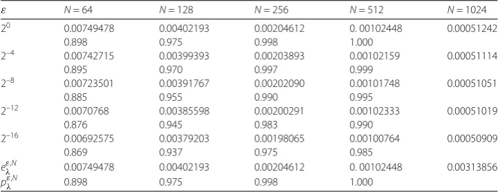
Table 2 Errorseελ,Ncomputedε-uniform errorseNλand convergence ratespελ,NonωN
ε N= 64 N= 128 N= 256 N= 512 N= 1024
20 0.00749478 0.00402193 0.00204612 0. 00102448 0.00051242
0.898 0.975 0.998 1.000
2–4 0.00742715 0.00399393 0.00203893 0.00102159 0.00051114
0.895 0.970 0.997 0.999
2–8 0.00723501 0.00391767 0.00202090 0.00101748 0.00051051
0.885 0.955 0.990 0.995
2–12 0.0070768 0.00385598 0.00200291 0.00102333 0.00051019
0.876 0.945 0.983 0.990
2–16 0.00692575 0.00379203 0.00198065 0.00100764 0.00050909
0.869 0.937 0.975 0.985
eελ,N 0.00749478 0.00402193 0.00204612 0. 00102448 0.00313856
pελ,N 0.898 0.975 0.998 1.000
5 Conclusion
We have considered the numerical approximations of a class of quasilinear singularly per-turbed first order parameterized differential problems with integral boundary conditions, which serves as the model for many scientific applications. For the numerical solution of this problem, we proposed a uniform convergent finite difference scheme on the graded Bakhvalov mesh. The ideas presented here can be easily applied for solving more compli-cated initial value problems for parameterized singularly perturbed equations with inte-gral boundary conditions, and the technique presented in the paper can also be applied to high-dimensional systems.
Competing interests
The author declares that they have no competing interests.
Authors’ contributions
All authors contributed equally to the manuscript. All authors read and approved the final manuscript.
Publisher’s Note
Springer Nature remains neutral with regard to jurisdictional claims in published maps and institutional affiliations.
Received: 20 December 2017 Accepted: 26 April 2018
References
1. Farrel, P.A., Hegarty, A.F., Miller, J.J.H., O’Riordan, E., Shishkin, G.I.: Robust Computational Techniques for Boundary Layers. Chapman Hall/CRC, New York (2000)
3. O’Malley, R.E.: Singular Perturbation Methods for Ordinary Differential Equations. Springer-Verlag, New York (1991) 4. Roos, H.G., Stynes, M., Tobiska, L.: Numerical Methods for Singularly Perturbed Differential Equations. Springer-Verlag,
Berlin (2008)
5. Na, T.Y.: Computational Methods in Engineering Boundary Value Problems. Academic Press, New York (1979) 6. Jankowski, T.: Application of the numerical-analytical method to systems of differential equations with a parameter.
Ukr. Math. J.54(4), 671–683 (2002)
7. Samoilenko, M., Martynyuk, S.V.: Justification of the numerical–analytic method of successive approximations for problems with integral boundary conditions. Ukrain. Mat. Zh. SSR43, 1231–1239 (1991)
8. Amiraliyeva, I.G., Amiraliyev, G.M.: Uniform difference method for parameterized singularly perturbed delay differential equations. Numer. Algorithms52, 509–521 (2009)
9. Amiraliyev, G.M., Amiraliyeva, I.G., Kudu, M.: A numerical treatment for singularly perturbed differential equations with integral boundary condition. Appl. Math. Comput.185, 574–582 (2007)
10. Amiraliyev, G.M., Kudu, M., Duru, H.: Uniform difference method for a parameterized singular perturbation problem. Appl. Math. Comput.175, 89–100 (2006)
11. Lui, X., Mcare, F.A.: A monotone iterative methods for boundary value problems of parametric differential equation. J. Appl. Math. Stoch. Anal.14, 183–187 (2001)
12. Pomantale, T.: A constructive theorem of existence and uniqueness for the problemy=f(x,y,λ),y(a) =α,y(b) =β. Z. Angew. Math. Mech.56, 387–388 (1976)
13. Feckan, M.: Parameterized singularly perturbed boundary value problems. J. Math. Anal. Appl.188, 426–435 (1994) 14. Jankowski, T.: One-step methods for ordinary differential equations with parameters. Apl. Mat.35(1), 67–83 (1990) 15. Turkyilmazoglu, M.: Analytic approximate solutions of parameterized unperturbed and singularly perturbed
boundary value problems. Appl. Math. Model.35, 3879–3886 (2011)
16. Amiraliyev, G.M., Duru, H.: A note on a parameterized singular perturbation problem. Appl. Math. Comput.182, 233–242 (2005)
17. Cen, Z.: A second order difference scheme for a parameterized singular perturbation problem. J. Comput. Appl. Math.
221, 174–182 (2008)
18. Das, P.: Comparison of a priori and a posteriori meshes for singularly perturbed nonlinear parameterized problems. J. Comput. Appl. Math.290, 16–25 (2015)
19. Kumar, S., Kumar, M.: A second order uniformly convergent numerical scheme for parameterized singularly perturbed delay differential problems. Numer. Algorithms76(2), 349–360 (2017)
20. Shakti, D., Mohapatra, J.: Layer-adapted meshes for parameterized singular perturbation problem. Proc. Eng.127, 539–547 (2015)
21. Xie, F., Wang, J., Zhang, W., He, M.: A novel method for a class of parameterized singularly perturbed boundary value problems. J. Comput. Appl. Math.213(1), 258–267 (2008)
22. Wang, Y., Chen, S., Wu, X.: A rational spectral collocation method for solving a class of parameterized singular perturbation problems. J. Comput. Appl. Math.233, 2652–2660 (2004)
23. Cannon, J.R.: The solution of the heat equation subject to the specification of energy. Q. Appl. Math.21(2), 155–160 (1963)
24. Iokin, N.I.: Solution of a boundary value problem in heat conduction theory with nonlocal boundary conditions. Differ. Equ.13, 294–304 (1977)
25. Nicoud, F., Schönfeld, T.: Integral boundary conditions for unsteady biomedical CFD applications. Int. J. Numer. Methods Fluids40, 457–465 (2002)
26. Ahmed, B., Khan, R.A., Sivasundaram, S.: Generalizedquasilinearization method for a first order differential equation with integral boundary condition. Dyn. Contin. Discrete Impuls. Syst.12, 289–296 (2005)
27. Borovykh, N.: Stability in the numerical solution of the heat equation with nonlocal boundary conditions. Appl. Numer. Math.42, 17–27 (2002)
28. Çakir, M.: A numerical study on the difference solution of singularly perturbed semilinear problem with integral boundary condition. Math. Model. Anal.21(5), 644–658 (2016)
29. Çakir, M., Amiraliyev, G.M.: Numerical solution of a singularly perturbed three-point boundary value problem. Int. J. Comput. Math.84(10), 1465–1481 (2007)
30. Cen, Z., Cai, X.: A second-order upwind difference scheme for a singularly perturbed problem with integral boundary condition in neutral network. In: Lecture Notes in Artificial Intelligence, vol. 4693, pp. 175–181. Springer, Berlin (2007) 31. Kudu, M., Amiraliyev, G.M.: Finite difference method for a singularly perturbed differential equations with integral
boundary condition. Int. J. Math. Comput. Sci.24(3), 72–79 (2015)
32. Bakhvalov, N.S.: On the optimization of the methods for solving boundary value problems in the presence of a boundary layer. USSR Comput. Math. Math. Phys.9(4), 139–166 (1969)
33. Kumar, S., Kumar, M.: Analysis of some numerical methods on layer adapted meshes for singularly perturbed quasilinear systems. Numer. Algorithms71(1), 139–150 (2016)
34. Amiraliyev, G.M.: The convergence of a finite difference method on layer-adapted mesh for a singularly perturbed system. Appl. Math. Comput.162(3), 1023–1034 (2005)