ABSTRACT
KANG, CHANGKU. Regression via clustering using Dirichlet mixtures. (Under the direction of Subhashis Ghosal.)
Regression via clustering using Dirichlet mixtures
by
Changku Kang
A dissertation submitted to the Graduate Faculty of North Carolina State University
in partial fulfillment of the requirements for the Degree of
Doctor of Philosophy
Statistics
Raleigh 2005
Submitted on : 10/06/2005
APPROVED BY:
Subhashis Ghosal John F. Monahan
Chair of Advisory Committee
Biography
Acknowledgements
Contents
List of Tables vii
List of Figures viii
1 Introduction 1
1.1 Overview . . . 1
2 Non-Bayesian and Bayesian Methods for Regression 8 2.1 Classical Methods . . . 10
2.1.1 Linear regression . . . 10
2.1.2 Nonparametric regression . . . 13
2.2 Bayesian Methods . . . 18
2.2.1 Gaussian process method . . . 18
2.2.2 Basis expansion method . . . 19
2.3 Other methods . . . 21
3 Preliminaries 23 3.1 Dirichlet process and Dirichlet mixture process . . . 23
3.2 Evaluation of clustering . . . 29
3.3 Inference about M . . . 31
3.4 Posterior consistency . . . 32
4 Dirichlet Mixture Regression 36 4.1 Estimation via MCMC sampling . . . 36
4.1.1 Estimation of Σand m,Φ . . . 39
4.1.2 The procedure of the estimation of E(Y|X) . . . 40
4.1.3 Merging clusters . . . 43
4.2 Confidence band for regression function . . . 43
5 Simulation study and Applications 54
5.1 One dimension . . . 55
5.2 Two dimension . . . 63
5.3 Higher dimension . . . 66
5.4 Large p, small n case. . . 73
5.5 Real data example . . . 77
6 Conclusions and Future Work 83
List of Tables
5.1 One dim: P-values of the paired t-test for performances . . . 60
5.2 One dim: P-values of the t-test for performances . . . 63
5.3 Two dim: P-values of the t-test . . . 64
5.4 Ten dim: The simulation numbers . . . 67
5.5 Ten dim: P-values of the t-test . . . 68
5.6 Ten dim: P-values of Wilcoxon test . . . 68
5.7 Ten dim: sparse model: P-values of the t-test . . . 69
5.8 Ten dim: sparse model: P-values of Wilcoxon . . . 69
5.9 Large psmall n: The simulation result . . . 75
List of Figures
1.1 The conditional mean and variance . . . 4
4.1 The partition of two dimensional space . . . 48
4.2 The plot of two and three mixtures . . . 53
5.1 One dim: the plot of data and fitted line . . . 56
5.2 One dim: L1-error Comparison . . . 58
5.3 One dim: L2-error Comparison . . . 59
5.4 One dim: the true is not linear . . . 61
5.5 One dim: True is not linear . . . 62
5.6 Two dim: data plot and similar measure . . . 64
5.7 Two dim: L2-error and risk Comparison . . . 65
5.8 Ten dim: L1-error Comparison . . . 70
5.9 Ten dim: sparse model - L1-error Comparison . . . 71
5.10 Ten dim: various tuning parameters in the LASSO . . . 72
5.11 Leukaemia data: The plot of Rand’s measure according to the choice of c . . . 76
5.12 Nonprofit organization data: The trace plot of the number of clusters 79 5.13 Nonprofit organization data: The trace plot of the number of clusters after mergin clusters . . . 79
5.14 Nonprofit organization data: The estimated value of donation . . . . 80
Chapter 1
Introduction
1.1
Overview
A common problem of data analysis in modern statistics is the estimation of a regression function based on sampled data (X1, Y1), . . . ,(Xn, Yn). The regression
subpopulations where different regression functions are in effect, but subpopulation membership is abstract and is not observable. Had we observed the labels, regression analysis would have been straightforward. In the absence of the labels, we use the auxiliary measurements to impute the labels and use simple regression analysis within each hypothetical group. It is not unreasonable to expect that subjects within similar measurement are likely to have similar background and mentality. If customers of dif-ferent types are identified, we may use simple regression analysis within each cluster and the true overall regression function will be estimated as a weighted combination of all regression estimates. In the whole analysis, uncertainty in group membership as well as the number of groups should be taken into consideration.
In this thesis we propose a method to estimate an unknown regression function by splitting it into an unknown number of clusters and then using some simple regres-sion models within each cluster. In finding the clusters, a Bayesian nonparametric method is considered. Standard regression methods are used in fitting a regression function within each cluster. We also give an intuitive argument why consistency of our estimator is expected.
Suppose we are given data (X1, Y1), . . . ,(Xn, Yn) whereXi isp-variate continuous
variables and Yi is univariate. We want to consider the regression model,
Yi =f(Xi) +εi, i= 1, . . . , n, (1.1)
where εi iid
∼ N(0, T2). It is not assumed that f(·) has a specific structure, such as
are, respectively, distributed as
N(µ1,Σ1), . . . , N(µk,Σk); (1.2)
hereµj is the mean vector and Σj is thep×pvariance covariance matrix corresponding
to the jth group. Let J be the latent variable which indicates the index of the group
where the observation belongs. The prior distribution ofJ is given byπj =P(J =j)
and thus the posterior distribution given that anX observation is equal tox is given by πj(x) = P(J =j|X = x). Let the conditional distribution of X given J and the
conditional distribution ofY given X and J be given by
X|J =j ∼N(µj,Σj), (1.3)
Y|X =x, J =j ∼N(fj(x), Tj2), j = 1, . . . , k,
wherefj(x) is the regression function in group j. Then, by the law of total
probabil-ities,
E(Y|X =x) =
k
X
j=1
E(Y|X =x, J =j)·P(J =j|X =x) =
k
X
j=1
fj(x)πj(x). (1.4)
Also, the conditional variance is given by
Var(Y|X =x) = EJ(Var(Y|X =x, J)) + VarJ(E(Y|X =x, J))
= EJ(TJ2) + VarJ(fJ(x))
=
k
X
j=1
Tj2πj+ k
X
j=1
fj2(x)πj(x)−
Xk
j=1
fj(x)πj(x)
2
. (1.5)
Note here that if T2
j are all equal, then first term in (1.5) is constant but the other
−2 −1 0 1 2
−2.0
−1.5
−1.0
−0.5
0.0
0.5
x
E( Y | X)
−2 −1 0 1 2
0.25
0.30
0.35
0.40
0.45
0.50
x
Var( Y | X)
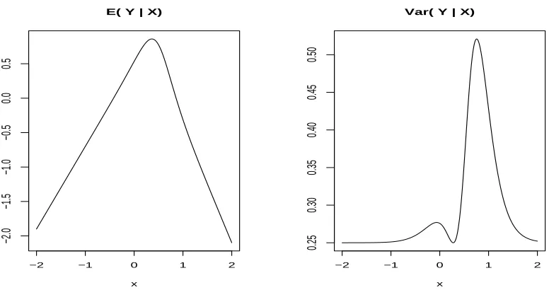
Figure 1.1: The plot of the conditional expectation and variance which depend on the value of X. X is distributed by the mixture of two normals with π1 =π2 = 0.5,
µ1 = 0, µ2 = 1, Σ1 = Σ2 = 0.42, f1(x) = 0.5 + 1.2x, f2(x) = 1.3 − 1.7x, and
T2
1 =T22 = 0.52.
may not be homoscedastic. This shows that usual nonparametric regression model is unable to handle this simple and intuitive structure in model (1.3). Of course heteroscedastic nonparametric model contains (1.3), but it is very difficult to estimate the regression function under that scenario.
The idea of estimation of the regression function in this situation has two steps. In the first step, as we assume that the underlying distribution ofX follows the mixture distribution, we may try to recover lost subpopulation labels by identifying clusters in the data. Second, once the clusters have been identified, standard parametric regression techniques may be used within each cluster.
Dirichlet mixture of normal prior for the density ofX observations which means that we model the density of X as a mixture of normal densities and true mixing dis-tribution given the Dirichlet process prior. Because Dirichlet samples are discrete distributions and observations arise according to a Polya urn scheme (see Chapter 3), the Dirichlet mixture prior has the ability to automatically produce clusters. The means of the hidden groups are generated by an MCMC algorithm. In fact, we only need the configuration of the ties among the latent means to identify the clusters at each MCMC step but the group means and hyperparameters need not be updated within MCMC iteration. This will allow substantial reduction of computational com-plexity at the MCMC step.
Once the clusters have been identified, we can use a standard regression method, such as the method of least squares for linear regression, within each cluster. Poly-nomial regression may be used if we suspect the lack of linearity in the model. In the multidimensional case, a parsimonious model building is an important issue so that a variable selection method is usually used in regression problems. A useful method which can automatically select the important variables while estimating regression is given by the LASSO regression method [Tibshirani (1996)]. Unlike other shrinkage methods such as the ridge regression [Hoerl and Kennard (1988)], LASSO can shrink certain coefficients to exactly zero depending on the value of some tuning parameter. A cross validation method can be applied to find the optimal value of the tuning parameter.
For instance, the inversion of high dimensional covariance matrix may be needed for the fully Bayesian method. Instead we use simple non-Bayesian estimates so that we can save substantial computing time.
There is a challenging problem, so-called the large p small n problem, where the number of variables p is large relative to the number of samples n. This happens in many applications such as the microarray data analysis. The method of least squares is inappropriate to handle this problem because of singularity while LASSO tends to have erratic behavior. We propose using the elastic net method suggested by Zou and Hastie (2005) and use it in each cluster to estimate parameters of each regression function after DM procedure finds the clusters.
We will compare our method with several nonparametric methods. A lot of meth-ods using local smoothing such as the kernel method and spline smoothing in the univariate case were provided by many authors. These methods can be applied when there is only one regressor variable. In the multivariate case, the data are sparsely distributed even for a large sample size. This well known difficulty is called “the curse of dimensionality”. Many standard nonparametric techniques suffer from this prob-lem. Therefore, it is necessary to consider certain approaches to overcome this kind of problem, especially in a high dimensional situation. Among the important non-parametric regression techniques in higher dimension are Multivariate Adaptive Re-gression Splines (MARS) [Friedman (1991)] and Generalized Additive Model (GAM) [Hastie and Tibshirani (1990)]. These methods are briefly described in Chapter 2.
evaluateL1-error andL2-error given in (5.1). These are common measures of distance
between true regression function and the estimated function in a global sense. An advantage of our method is that there is no need to select to the bandwidth parameter. In the Dirichlet mixture model in (3.1), we need to specify constant M, distribution G0 and prior for σ. The parameter M is called “precision parameter” because of its
role in controlling the spread of the Dirichlet process. We can specify the prior forM but a fixed small value is used here. The posterior distribution of k only depends on the number of clusters in certain MCMC steps so we can easily update and get the information ofk. In fact, the value ofk obtained from MCMC step is an overestimate of the number of clusters. But, this does not harm much in estimating the regression function; see explanations given in Section 5.3.
Chapter 2
Non-Bayesian and Bayesian
Methods for Regression
In this chapter we review the literature about the regression method from the non-Bayesian and Bayesian nonparametric perspectives. Suppose that there are a vector X = (X1, . . . , Xp) and a real valued random variable Y of interest which is
influenced byX. Regression describes the approximate relationship betweenXandY given data (X1, Y1). . . ,(Xn, Yn) where Xi = (Xi1, . . . , X
p
i). The variable X is called
the independent or predictive variable and Y is called the dependent or response variable.
The general heteroscedastic regression model is defined by
Yi =f(Xi) +εi, (2.1)
where εi is usually assumed by the independent normal distribution having mean 0
and variance σ2
on the covariate vector X. If the functional form of f(·) such as linearity is not given, then the model is nonparametric. The simplest and most popular one is the homoscedastic linear regression as a parametric regression by assuming f(x) = Xβ and σ2
i(x) = σ2. In our problem, we focus on using linear regression within each
cluster after finding several candidate groups.
The ordinary least squares (OLS) method is very popular and a simple method of estimation in linear regression models. We begin with a review of the linear regression along with its modification such as the ridge regression and the LASSO method. Then nonparametric regression method will be reviewed. This method has certain difficulty in the multidimensional case, known as “the curse of dimensionality”. Several meth-ods were developed to overcome this drawback. A generalized additive model (GAM) is suggested to restrict the form of the function and multivariate adaptive regression splines (MARS) is developed as the generalization of recursive partitioning regression model.
2.1
Classical Methods
2.1.1
Linear regression
The simplest regression model is the linear regression which assumes that regres-sion function is a linear function ofX. Assume that we have the regression model in (1.1). The linear regression model assume f(·) has the linear structure
Yi = p
X
j=0
Xijβj +εi, (2.2)
where εi is distributed by the independent normal distribution having mean 0 and
varianceσ2 andX
i0 = 1 for alli= 1, . . . , n. We may assume thatXi’s are distributed
according to a certain distribution such as a normal distribution. The regression function can be expressed as the conditional expectation ofY givenX,E(Y|X). This model includes the polynomial regression model. For example, ifXis univariate, then by defining X2 =X12 quadratic relationship can be incorporated into by the model.
Let X be the n×(p+ 1) matrix with (i, j)th component as X
i,j and similarly let
Y be the column vector of length n whose ith entry Y
i. Then, model (2.2) can be
expressed as
Y =Xβ+ε, (2.3)
where β = (β0, . . . , βp)T and ε = (ε1, . . . , εn)T. The OLS estimator is obtained by
minimizing the sum of squared error (SSE)
SSE (β) = (Y−Xβ)T(Y−Xβ), (2.4) leading to the solution
b
Note that here we have assumed that XTX is a non-singular matrix. If the design
matrix XTX is singular, we can use a generalized inverse of XTX.
The Gauss-Markov theorem states that OLS estimator has the minimum variance among any other unbiased linear estimators. However, OLS method suffers in pre-diction particularly if XTX is singular or near singular. The prediction error can be
improved by reducing variance but allowing some bias. Ridge regression and LASSO regression are penalization techniques applied to the model.
Ridge regression, introduced by Hoerl and Kennard (1970), penalizes the size of the regression coefficient. The estimate is obtained by minimizing the penalized sum of squares,
SSE (β, λ) = (Y−Xβ)T(Y−Xβ) +λβT
β, (2.5)
where λ is a complexity parameter that controls the amount of shrinkage. If λ in-creases to infinity, the amount of shrinkage is larger. Now the solution of (2.5) is,
b
βridge = (XTX+λI)−1XTY, (2.6)
where I is the (p+ 1)×(p+ 1) identity matrix. Equivalently the ridge coefficient minimizes the usual SSE in (2.4) subject to the constraint that Ppj=0β2
j ≤ s, where
s is the parameter playing the same role of λ. The difference between the ridge coefficients and OLS coefficients is λ times the identity matrix added to XTX. In
fact, (XTX+λI) is not singular even if XTX is a singular matrix. ForXTX nearly
singular, Var(βbridge) can be substantially lower than Var(βbOLS). This is the main motivation behind ridge regression.
LASSO, introduced by Tibshirani (1996), minimizes SSE subject to a bound on the L1-norm. Unlike the ridge regression, the LASSO can make some coefficients exactly
zero so that we can choose a subset of the predictors which have relatively stronger effect on the dependent variableY. There is a discrete variable selection procedure so called best subset. However, the LASSO method works both as a continuous shrinkage and an automatic variable selection technique. Similar to the ridge method, the LASSO coefficients can be defined that minimizes the SSE subject to Ppj=0|βj| ≤s.
Tibshirani (1996) and Fu (1998) compared above methods in terms of prediction error but there is no one which is superior to the other method. Recently, Zou and Hastie (2005) developed a method which combined the ridge regression and LASSO to give what is called the “elastic net (EN)” and used in microarray data analysis. Especially EN outperforms the LASSO when the number of predictors, p, is much larger than the number of observations,n, (“the largep, smalln” problem) and when there is a group of highly correlated variables.
2.1.2
Nonparametric regression
The linear regression model has the advantages of simple interpretation and easy computation. But, it has a limited flexibility and produces accurate estimates only when the true form of the regression function is close to the linear function. This motivates the use of more flexible models.
Univariate case
On estimation of nonparametric regression function there are roughly three para-digms such as local parametric, piecewise fitting and roughness penalty method.
• Local parametric fitting : There are two main issues in this method. One is how big the neighborhoods are and the other is how to average the target value in each neighborhood. Bin smoother, which is also known as “regressogram” is a basic method like histogram for density estimation. If we use the least square method in a neighborhood then the running line method is obtained. A useful and popular estimator is the kernel estimator proposed by Nadaraya (1964) defined by
b f(X) =
Pn
i=1Kh(X−Xi)Yi
Pn
k=1Kh(X−Xk)
, (2.7)
whereKh(·) = 1hK(h·) is a kernel function having bandwidthh >0 and K(·) is
a symmetric density function. It is useful to represent this in matrix notation.
b
f(X) =SY, where Si,j =
Pn
i=1Kh(Xj −Xi)
Pn
k=1Kh(X−Xk)
, (2.8)
matrix. For the method of least squares, the smoother matrix is nothing but the hat matrix H=X(XTX)−1XT. This representation also applies to smoothing
splines and other nonparametric methods.
There may be many choices for the kernel functions but it is known that the choice of bandwidth h is more important than that of the kernel function. A common choice for the kernel function is the standard normal distribution. A common method for bandwidth selection is that of cross validation (CV). For given data (X1, Y1), . . . ,(Xn, Yn), for i = 1, . . . , n, we leave (Xi, Yi) out and fit
the estimate off, say fb(−i) then calculate the error as
CV = 1 n
n
X
i=1
Yi−fb(−i)(Xi)
2
= 1 n
n
X
i=1
Yi−fb(Xi) 1−Si,i
2
,
where Si,i is the diagonal elements of the smoother matrix S. Note here, fb(−i)
and fbdepend on the bandwidth h. The optimal h can be obtained by min-imizing CV. Alternatively generalized cross validation (GCV) is proposed by replacing Si,i by 1n tr(S). Craven and Wahba (1979) proposed GCV method
and established the optimal property of GCV. In this thesis, we will use the method which was proposed by Sheather and Jones (1991). This is already implemented in R package, “KernSmooth” with function “dpik” and “ksmooth”.
order of polynomial at each subregion. The main difficulty is to select the order of polynomial as well as the knots. Splines can be represented by different basis functions. For example, cubic regression splines can be expressed by the following.
b
f(x) =β0+β1x+β2x2+β3x3+
N
X
j=1
θj(x−ξj)3+, (2.9)
where ξ1, . . . , ξN are given knots and (a)+= max(a,0).
• Roughness penalty method : A Sobolev space is defined as a normed space of functions for which derivatives upto a certain order satisfy some integrability restrictions. Let f(x) be a function in the second order Sobolev space on unit interval, W2[0,1], then a smoothing spline is a function f ∈ W2[0,1] which
minimizes
1 n
n
X
i=1
Yi−f(Xi)
2
+λ Z 1
0
f′′(x)2dx, (2.10) where λ > 0 is a smoothing parameter. The second term of (2.10) penalize the roughness or the curvature of estimator. The parameter λ controls the bias-variance trade off. For example, if λ = 0, the f(Xb i) = Yi and if λ = ∞
then fbis the least square regression line. The solution of (2.10) is called cubic spline with knots X1, . . . , Xn. It is important to chooseλ properly. The
Multivariate case
Nonparametric regression method is challenged in the multidimensional case be-cause of the curse of dimensionality, which means that in high dimensions, a neighbor-hood containing a fixed percentage of data points can be very big. There have been many studies to overcome this difficulty. Mostly, a dimension reduction technique is considered and then smoothing methods are used even though there are direct smoothing approaches such as thin-plate spline and classification and regression trees (CART). Here we review some of recent methods such as the generalized additive model (GAM) and multivariate adaptive regression splines (MARS).
The additive model is a generalization of the usual linear regression model, where the regression function is assumed to be a sum of functions on lower-dimensions. The additive model is defined as
Yi = p
X
j=1
fj(Xj,i) +εi, i= 1, . . . , n, (2.11)
where εi iid
∼ N(0, T2). Note that f
j’s are arbitrary univariate functions, one for each
predictor. Hastie and Tibshirani (1990) adapted this additive model to generalized linear models, and this is called the generalized additive model (GAM). The GAM differs from a generalized linear model in that an additive part replaces the linear predictor. The GAM is defined as
g(µ) =
p
X
j=1
fj(Xj), (2.12)
local scoring procedure plays a role as the iteratively reweighted least square method in a generalized linear model. In R, “gam” function is implemented in the package “mgcv”. Since it is necessary to use the nonparametric estimation method to estimate each functionfj, the bandwidth parameters are selected by some suitable data driven
methods. In R, “gam” function uses the generalized cross validation method to select the bandwidth parameter.
MARS is a method for flexible modeling in high dimensional data, motivated from the recursive partitioning model by Friedman (1991) . This does not assume any parametric form off(X). MARS constructs the function from a set of coefficients and basis functions only from the data. The model is defined by
Yi =β0+
M
X
m=1
βmBm(Xi) +εi, i= 1, . . . , n, (2.13)
where Bm is a basis function. For example, suppose we consider the class,
C={(Xj −t)+,(t−Xj)+|t∈ {X1,j, . . . , Xn,j}, j = 1, . . . , p},
where (s)+=s if s >0, 0 otherwise. ThenBm is either a function in C or a product
2.2
Bayesian Methods
2.2.1
Gaussian process method
A Gaussian process is a collection of random variables and the finite number of which have joint normal distributions. A Gaussian process can be specified by the mean function m(x) and covariance function K(x, x′). Let f(x) denote the regres-sion function distributed as a Gaussian process (GP) with mean function m(x) and covariance function K(x, x′), then f ∼ GP(m, K). The choice of an appropriate co-variance function enables to have a large support in the space of all smooth functions. For example, the covariance functionK(x, x′) = 1
τe
−γ(x−x′)2
with varying γ spans the space of all smooth functions. The weak but crucial assumption for the covariance function is that it generates non-negative definite matrix for any set of inputs.
Suppose we have given data (X1, Y1), . . . ,(Xn, Yn) and we want to predict the
estimate off(xn+1) at givenxn+1. Letf = (f(X1), . . . , f(Xn))T andm= (m(X1), . . . ,
m(Xn))T and Σ0 the covariance matrix having the (i, j)th element K(Xi, Xj). The
conditional distribution off given data is
f|(X1, Y1), . . . ,(Xn, Yn)∼GP(m∗, K∗), (2.14)
where
m∗(x) = m(x) +K(x,X)TΣ−01(f −m), K∗(x,X) = K(x, x)−K(x,X)TΣ−1
0 K(x,X),
and K(x,X) = (K(x, X1), . . . , K(x, Xn))T. The above expression is easily obtained
multi-variate normal distribution, and the distribution of f(xn+1) is the conditional
distri-bution from the joint normal.
Now the specification of hyper parameters such as putting a prior forτ, γ in above example covariance function gives us posterior updating formula. An MCMC method is considered by Neal (1997) and MacKay (1999). One difficulty for this method is its long computing time, as the covariance function, which depends on the data size needs to be inverted. Before modern cheap and fast computing machine it was not feasible to compute the inverse of matrix whose dimension is more than hundred. But, now it is feasible to apply this method in the case of more than thousands of samples. The strength of GP method is the conceptual simplicity and the flexibility in modeling. Rasmussen (1996) has compared GP with other nonparametric regression methods and shown that GP has better performance among them. Geostatistics is a common application area of GP, where the predictor is of two or three dimensions [Cressie (1993)]. Choi and Schervish (2004) established the posterior consistency of Gaussian process priors for the regression function in normal error case in one dimension.
2.2.2
Basis expansion method
Many Bayesian methods for nonparametric regression problem use some basis expansion such as splines, the Fourier basis and wavelet bases. Suppose that given a basis {f1, . . . , fM}, the regression function can be expressed by
f(·) =
M
X
j=1
bjfj(·), (2.15)
Splines commonly use basis functions as
{1, x, x2, x3,(x−ξ1)+3, . . . ,(x−ξp)3+}, (2.16)
where (x)+ = max(x,0) and ξ = (ξ1, . . . , ξp) is a vector of knots. For a given ξ, the
regression function can be formed by the coefficients b= (b1, . . . , bM). The
specifica-tion of prior for (ξ, b, σ) enable to set up a Bayesian model in this problem. There are many approaches depending on different priors on b (see Section 3.1 in Muller and Quintana (2004)). Updating ξ, a vector of knots, is somewhat difficult when the number of knots and locations are unknown. Denison et al. (1998) proposed a procedure which enables to add, delete and change knots from the data by using the reversible jump MCMC method. For the multivariate case, the additivity assump-tion is common. Denisonet al. (1998) assumed the additive structure. Alternatively, Denison et al. (1998b) proposed Bayesian approach to MARS by using the reversible jump MCMC method. They showed that Bayesian MARS have a high predictive power due to posterior averaging.
Wavelet basis methods provide an orthonormal L2 basis of the space of square
integrable functions. AnyL2 functionf can be represented by the wavelet expansion,
f(x) =X
j
X
k
dj,kψj,k(x), (2.17)
with basis functionψj,k(x) = 2
j
2ψ(2jx−k). This representation is usually very sparse
so that there are only a few coefficients having relatively large values. The idea is to first consider the discrete wavelet transform from given data and then discard those small coefficients by thresholding. With those coefficients, one can reconstruct the original data by the inverse of discrete wavelet transformation. Let d∗
empirical coefficients obtained by applying discrete wavelet transform to the data (Y1, . . . , Yn). Then, Bayesian wavelet regression methods need to get the posterior
distribution of dj,k|d∗j,k by putting a prior on dj,k. Chipman et al. (1997) put an
independent prior on dj,k,
dj,k|γj,k ∼γj,kN(0, c2jνj2) + (1−γj,k)N(0, νj2),
where γj,k ∼Bernoulli(pj) and all the hyperparameters are determined by empirical
methods. Then, the posterior distribution is also a mixture of two normal distribu-tions because d∗ has a normal distribution with mean d
j,k and a fixed variance.
Abramovich et al. (1998) placed independent priors on dj,k as
dj,k ∼pjN(0, τj2) + (1−pj)δ(0),
where δ(0) is degenerate probability at 0. Vidakovic (1998) proposed a mixture of a point mass and a t−distribution. Holmes and Denison (1999) considered an infinite mixture of normals.
2.3
Other methods
Muller, Erkanli and West (1996) suggested a nonparametric Bayesian curve fitting method. Their idea is that once the distribution of joint density (X, Y) is known then the conditional distribution of Y|X can be easily obtained. The joint distribution of (X, Y) is assumed to be a mixture. Dirichlet mixtures of normals prior was used to estimate the joint distribution. Their method is a fully Bayesian method. The method suffers in higher dimensional case and the large p small n problem and also when the conditional mean is not linear in each subpopulation.
Chapter 3
Preliminaries
In this chapter we review Bayesian nonparametric method concepts such as the Dirichlet process, and the Dirichlet mixture process and their properties. The poste-rior is typically computed using the MCMC method of Gibbs sampling. The MCMC sampling scheme and the consistency of posterior distribution will be reviewed in this chapter.
3.1
Dirichlet process and Dirichlet mixture process
whose sample paths are probability measures, is the Dirichlet process introduced by Ferguson (1973).
Let M(X) be the space of probability measure on X. Let G be a probability measure on (X,B) whereB is the Borel σ-field.
Definition 1 Let M > 0 and G be a probability measure on (X,B). A random probability measure P follows a Dirichlet process on (X,B) if for any finite partition
{B1, . . . , Bk} of X, the joint distribution of the vector (P(B1), . . . , P(Bk)) has the
Dirichlet distribution with parameter (M G(B1), . . . , M G(Bk)).
The Dirichlet distribution for variables (x1, . . . , xk) with parameter (p1, . . . , pk) is
defined by
f(x1, . . . , xk) =
1 C
k
Y
i=1
xpi−1
i ,
when x1, . . . , xk ≥ 0, Pki=1xi = 1 and p1, . . . , pk > 0. The constant C is given by
Qk
i=1Γ(pi)/Γ(Pki=1pi), where Γ(·) is the gamma function. We denote “DP(M, G)”
as the Dirichlet process with parameter (M, G). Note here,
E(P(B)) = G(B), Var(P(B)) = G(B)(1−G(B))
1 +M . (3.1)
If M gets larger, then P approachesG. The number M is called the precision para-meter and Gis called the center measure, andM Gis referred to as the base measure ofDP(M, G). An attractive mathematical property of Dirichlet process is that given a set of realizations θ1, . . . , θn from P ∼DP(M, G0), the posterior distribution of P
is also a DP(M∗, G∗0) whereM∗ =M+n andG∗0 = (M G0+Pni=1δθi)/(M+n); here
scheme model which also gives a construction of the Dirichlet process [Blackwell and MacQueen (1973)].
θ1 ∼ G0 (3.2)
θi|θ1, . . . , θi−1 ∼
M G0+Pij−=11δθj
M +i−1 , for i= 1,2, . . . .
Therefore the predictive distribution of θn+1 can be derived by the following
θn+1|θ1, . . . , θn ∼
M
M +nG0+ 1 M+n
n
X
i=1
δθi. (3.3)
Sethuraman (1994) gave a useful construction of Dirichlet process. Suppose P is fromDP(M, G). Then
P = ∞ X
i=1
Viδθi, (3.4)
where θ1, θ2, . . . are a sequence i.i.d. random variable from G, Vi = Yi
Qi−1
j=1(1−Yj)
and Y1, Y2, . . . are i.i.d. random variables from Beta(1, M). Thus probabilities are
assigned by “stick breaking” at randomly distributed points. It can be easily shown that P∞i=1Vi = 1 almost surely. With this definition of Dirichlet process, we can
generate a realization of the Dirichlet process by truncation at some finite stage. It follows that Dirichlet process is almost surely discrete.
The weak support of Dirichlet process, DP(M, G) can be shown to be {P ∈
M(X) : supp(P) ⊂ supp(G)}. This means that if the support of G is X, then the space of all probability measures is the support of P. For example, if we have normal distribution as G, then the Dirichlet process can choose any probability measure.
Suppose that X1, . . . , Xn are drawn as a random sample from the distribution of
f(·, G) = Z
K(·, θ, σ)dG(θ), (3.5)
where K(·, θ, σ) is a density function given θ, σ and G∼ DP(M, G0). This was
de-veloped by Ferguson (1983) and Lo (1984), and is called “Dirichlet mixture process”. The kernelK(·, θ, σ) can be any density function. The normal distribution with mean θ and variance σ2 is a common choice and we will work with this one. Note that we
can put the Dirichlet prior on the distribution of θ or (θ, σ2). In the latter case, the
center distribution G0 is the joint distribution of (θ, σ2). If we consider the Dirichlet
prior on the meanθ, then the normal Dirichlet mixture process model is
f(·, G) = Z
N(·;θ, σ2)dG(θ), (3.6)
where N(·;θ, σ2) is the p.d.f. of normal distribution with mean θ and variance σ2.
There is an alternative useful representation in terms of a hierarchical model, given below:
Xi|θi
ind
∼ N(·;θi, σ2), (3.7)
θi|G iid
∼G,
G∼DP(M, G0).
In Bayesian inference, we get the posterior distribution of all the parameters that we are interested in. The joint distribution of (θ1, . . . , θn, σ2) is not analytically tractable,
Suppose we are interested in sampling θ = (θ1, . . . , θn) from the distribution
π(θ). Let θ−i = {θj;j 6= i} for i = 1, . . . , n. Assume that the full conditional
distributions π(θi|θ−i) are given and it is easy to sample from it.
(i) Set initial valuesθ(0) = (θ1(0), . . . , θn(0)).
(ii) Obtain a new valueθ(j) = (θ1(j), . . . , θn(j)) fromθ(j−1)through succesive sampling
θ1(j) ∼ π(θ1|θ2(j−1), . . . , θ(
j−1)
n ),
θ2(j) ∼ π(θ2|θ1(j), θ
(j−1)
3 . . . , θ(nj−1)),
...
θn(j) ∼ π(θn|θ1(j), . . . , θ(nj−)1). (3.8)
(iii) Increase the counterj toj+ 1 and repeat the step (ii) until certain convergence rule is satisfied.
The Gibbs sampler is a very powerful algorithm and its implementation is often easy in many complex problems. According to the Gibbs sampler, we only need to obtain the conditional distribution of θi given θ−i,X and σ2. The following gives the basic
idea on how to implement MCMC steps in a Dirichlet mixture model.
Algorithm (1).
θi|θ−i, σ2,X ∝qi0Gi(θi) +
X
j6=i
qijδθj(θi), (3.9)
where
qi0 ∝
Z
qij ∝N(Xi;θj, σ2), n
X
j=1
qij +qi0 = 1,
Gi(θi)∝N(Xi;θ, σ2)dG0(θ).
Since there are many ties during the updating ofθi, the above algorithm is not efficient
and an alternative algorithm is usually considered. Let φ be the set of distinct θi’s
and letk be the number of distinct elements ofθ1, . . . , θn. Let s= (s1, . . . , sn) be the
configuration vector defined by
si =j if and only if θi =φj, i= 1, . . . , n j= 1, . . . , k.
LetH ={I1, . . . , Ik}be a cluster which is defined by
Ij ={i:si =j}.
Therefore, H is a partition of I ={1, . . . , n}. Now given the configuration vector s and φ,θ and H are uniquely determined by the following rule.
φ1 = θ1
φj = θi, if j ≥2 and i= min{m:θm 6=φ1, . . . , θm 6=φj−1} (3.10)
Let the following be the notations when the observationi is removed:
• θ−i ={θj : 1≤j ≤n, j 6=i},
• k−i: the number of clusters formed by θ−i,
• φ−i : the set of distinct observations among θ−i,
The following is the alternative simplified algorithm for (3.9); (θi|θ−i, σ2,X)∝qi0Gi(θi) +
X
φk∈φ−i
n−i,kqikδφk(θi), (3.11)
where qik∝N(Xi|φk, σ2).
It is known that above algorithm is not efficient because there is a small chance to have a new value of θ during procedure. There is a technique of “remixing” the φj after every step to prevent this problem. The vector of (θ1, . . . , θn) can be
fully determined by knowing the configuration vector (s1, . . . , sn) and distinct values
(φ1, . . . , φk). Therefore sampling θi is equivalent to sampling si and φi given s, φ−i,
i= 1, . . . , k. Note here that if si =j ≤k−i, then the newθi =φj and if si =k−i+ 1,
then let the new value θi be sampled from Gi. This gives an alternative and more
efficient updating procedure.
Algorithm (2).
Under the notation of (3.11), the distribution ofsi is
P(si =j|s−i, φ−i,X) ∝ n−i,jN(Xi;φj, σ2),
P(si =k−i+ 1|s−i, φ−i,X) ∝ M
Z
N(Xi;θ, σ2)dG0(θ), (3.12)
and the posterior distribution of φ1, . . . , φk are
P(φj|s,X)∝dG0(φj)
Y
i∈Ij
N(Xi;φj, σ2) for j = 1, . . . , k. (3.13)
3.2
Evaluation of clustering
from Dirichlet process can give us a “good” partition. Now the question is how the clustering is good? According to Rand (1971), an objective criterion should have the following three basic properties. First, clustering is discrete, that is every point is assigned to a specific cluster. Second, clusters are defined just as much by those points which they do not contain as by those points which they do contain. Third, all points are of equal importance in the determination of clustering.
Given n points, θ1, . . . , θn and two clustering vectors, s = {s1, . . . , sk1} and s
′ = {s′
1, . . . , s′k2}, define a measure d be defined by
d(s,s′) = Pn
i<jγij n
2
, (3.14)
where
γij =
1, if there existk and k′ such that both θ
i and θj are in both sk and s′k′,
1, if there existk and k′ such thatθ
i is in both sk and s′k′ while θj
is in neithersk or s′k′,
0, otherwise.
(3.15) In practice, we use a simple computational formula for d:
d(s,s′) =hn 2
−0.5(X
i
(X
j
nij)2+
X
j
(X
i
nij)2) +
X X n2iji/
n 2
, (3.16)
where nij is the number of points simultaneously in the ithcluster of s and the jth
3.3
Inference about
M
In MCMC updating scheme, a suitable choice of M is important because M controls the number of clusters,k. We may put a value for M as an initial moderate choice and a prior on M lets the data choose the appropriate M. In this section we review the distribution of k. The aim is to give the posterior distribution of M so that we can update during MCMC procedure. This approach originally came from Escobar and West (1995). There are alternative ways to put a prior on M. Escobar (1994, 1998) used a discrete probability on a suggested grid points. Liu (1996) showed how to obtain the maximum likelihood estimate of M.
The distribution of the number of component k is the following:
P(k|M, n) =Cn(k)·n!·Mk·
Γ(M)
Γ(M +n), (3.17)
where Cn(k) = P(k|M = 1, n). The expectation of k is given by
E(k) =
n
X
i=1
M
M +i−1 ≈Mlog
M +n M
. (3.18)
Then, we can obtain the posterior of M given data X,
P(M|k, θ,X) = P(M|k) (∵the independence of M, θ, and X given k) ∝ P(M)·P(k|M)
∝ P(M)·n!·Mk· Γ(M)
Γ(M+n) (∵Cn(k) does not depend on M) ∝ P(M)MkB(M, n)
= P(M)Mk
Z 1
0
whereB(a, b) = Γ(a)Γ(b)/Γ(a+b). Then, P(M|k) can be considered as the marginal distribution from a joint for M and a continuous quantity η such that
P(M, η|k)∝P(M)·MkηM−1(1−η)n−1, M > 0, 0< η <1.
Thus, ifP(M) =Gamma(a, b), then the posterior ofM is
P(M|η, k) ∝ Ma−1e−bMMkηM−1
∝ Ma+k−1e−M(b−logη)
= Gamma(a+k, b−logη). (3.20)
These distributions are well defined for all gamma priors and
P(η|M, k)∝ηM−1(1−η)n−1, 0< η <1.
Therefore in MCMC sampling steps, repeating to sample η and M will give us an appropriate value of M. Now, the estimated posterior distribution of M can be obtained by the following:
P(M|Data)≈ 1 N
N
X
i=1
P(M|ηi, ki) (3.21)
where ηi are the sample values of η.
3.4
Posterior consistency
from the data eventually dominates whatever prior information was. We will briefly illustrate some preliminary definitions and give an argument which indicates poste-rior consistency in the Dirichlet mixture model. Formally speaking, let Πn be the
posterior given samplesX1, . . . , Xn. Then Πnis consistent atθ0 if Πn(U)→1 a.s. for
every neighborhoodU ofθ0. It is equivalent to Πn w
→δθ0, “w” denotes convergence of
measures in the weak sense. Naturally, posterior consistency depends on the topology on the parameter space.
A fundamental theorem is given by Schwartz (1965) but it seems to be difficult to apply her theorem to our regression problem directly. We shall extend the consis-tency property in Dirichlet mixture of normal model of Ghosal et al. (1999) to the multivariate case. At present the weak consistency result is only proved. A result from Donoho (1988) showed that the number of mixture is a lower semi-continuous functional indicating that asymptotically the number of clusters produced by the Dirichlet mixture is at least equal to the number of components in the true mixture distribution. This will be discussed in Chapter 4.
Consistency under two topologies, the weak topology and the strong topology will be discussed in this chapter. We first give some definitions of neighborhoods on the space of all density functions. Let F be the space of all densities on R with respect to the Lebesgue measure. On F, the weak topology and the norm topology can be considered as natural topologies. Since a topology can be formed by defining the system of neighborhoods, we can start by giving two natural types of neighborhoods.
form:
n
f ∈F: Z
ψif −
Z ψif0
< ε for i= 1, . . . , ko, (3.22)
where ψi are bounded continuous functions on R. This topology is called “weak
topol-ogy”.
A strong neighborhood is a set containing a set of the form:
{f ∈F:kf−f0k< ε},
where k · kdenotes a metric.
Definition 3 A prior Π is said to be weakly consistent at f0, if
Π(U|X1, . . . , Xn)→1
with probability 1 for all weak neighborhoods U of f0.
The closeness between two functions can be measured by a metric, norm and so on. One such measure is the Kullback-Leibler divergence.
Definition 4 (K-L divergence) The Kullback-Leibler divergence between two
den-sities f, f0 is given by
K(f0, f) =
Z
f0(x) log
f0(x)
f(x)dx.
Definition 5 (K-L support) For any f0 ∈F, the Kullback-Leibler neighborhood of
radius ε around f0, is given by Kε(f0) = {f :K(f0, f)< ε}.
Let Π be a prior on F, we say that f0 is in the K-L support of Π if
Theorem 1 [Schwartz (1965)]. If f0 is in the K-L support ofΠ, then the posterior
is weakly consistent at f0.
For the strong consistency, Barron, Schervish and Wasserman (1999) used the Hellinger bracketing entropy while Ghosalet al. (1999) usedL1-metric entropy which
gives a condition weaker than Barron et al. (1999).
Theorem 2 [Ghosal et al. (1999)]. Suppose f0 is in the K-L support of the prior
Π and for every ǫ >0 there exists a δ < ǫ, c1, c2 >0, β < ǫ2/2 and Fn such that
(i) Π(Fc
n)< c1e−nc2,
(ii) J(δ,Fn)< nβ, where J(δ,Fn) is the logarithm of the minimal number of balls
of radius δ in the total variation metric needed to cover the Fn.
Then the posterior is consistent in the total variation distance.
Chapter 4
Dirichlet Mixture Regression
In this chapter we show how to implement our proposed method to estimate the regression function under the mixture structure. It includes the specification of up-dating scheme of posterior using Gibbs sampling method and upup-dating corresponding of hyperparameters. However, we do not actually update the hyperparameters; rather we replace by the empirical estimates. We do this to minimize computational com-plexity. Some theoretical results based on certain well known theorems about the Dirichlet mixture model will also be presented along the sequel.
4.1
Estimation via MCMC sampling
Suppose that we have the following model.
Xi|θi
ind
∼ N(θi,Σ), i= 1, . . . , n
θi|G iid
G∼DP(M, G0), (4.1)
where G0(θ) =φ(θ;m,Φ) is a p.d.f. of multivariate normal distribution with mean
vector mand covariance matrix Φ.
Note here, the center measure is considered to have hyperparameters m and Φ. In this way we can expect a more flexible model compared to using a fixed center measure. The p−variate case is considered here since it includes the univariate case.
Then,
θi|θ−i,X ∼q0,iGi(θi) +
X
qj,iδθj(θi), (4.2)
where
qj,i ∝φ(Xi;θi,Σ),
q0,i∝M
Z
φ(Xi;θi,Σ)dG0(θ),
X
j6=i
qj,i+q0,i = 1,
and Gi(θi) is the posterior distribution of θi given Xi with the prior G0(θi) and the
likelihood N(θi,Σ). That is,
dGi(θi)∝φ(θi;Xi,Σ)φ(θi;m,Φ).
There is also another equivalent form of (4.2).
θi|θ−i,X ∼q0,iGi(θi) +
X
φk∈φ−i
n−i,kqk,iδφk(θi).
Given the assumptions in (4.1), the distribution of si given s−i, θ∗−i and X is the
Let θ∗ be the vector of the distict value of θ. For j = 1, . . . , k−
i,
P(si =j|s−i, θ−∗i,X) ∝ n−i,jφ(Xi;θ∗j,Σ),
P(si =k−i+ 1|s−i, θ−∗i,X) ∝ M
Z
φ(Xi;θ∗,Σ)dG0(θ∗). (4.3)
Since it is useful to consider only the update of s rather than s and θ∗ both, we can integrate out θ∗
j from the above theorem.
Algorithm (3)
Given the assumptions in (4.1), the distribution ofsi givens−i andX is the following:
Forj = 1, . . . , k−i,
P(si =j|s−i,X) ∝ n−i,j
Z
φ(Xi;θ∗,Σ)dH−i,j(θ∗),
P(si =k−i+ 1|s−i,X) ∝ M
Z
φ(Xi;θ∗,Σ)dG0(θ∗)
∝ M φ(Xi;m,Σ+Φ), (4.4)
where H−i,j is the posterior distribution based on the prior G0 and all observations
Xl for which l ∈Ij and l 6=i. That is,
dH−i,j(φ) =
1 Ci,j
h Y
l∈Ij,l6=i
φ(Xl;θ∗,Σ)
i
dG0(θ∗),
where Ci,j is the normalizing constant.
Note that here, the above formula can be simplified by using certain updating equation. The first quantity can be expressed as the following:
Z
φ(Xi;θ∗,Σ)dH−i,j(θ∗) =
R
φ(Xi;θ∗,Σ)
h Q
l∈Ij,l6=iφ(Xl;θ
∗,Σ)iφ(θ∗;m,Φ)dθ∗ R h Q
l∈Ij,l6=iφ(Xl;θ
The only difference between the numerator and denominator is in the termφ(Xi;θj∗,Σ)
which is additional in the numerator. When we add or delete one datum from the original, we can easily update the sample mean and sample variance without recom-puting the same for the whole data except the deleted observation. This should be helpful in calculating above ratio of two integrals. The result is again the ratio of two normal p.d.f.’s which is multiplied with another normal p.d.f. The equation of (4.5) can be written as
n−i,j
n−i,j+ 1
φ(Xi;X+i,j,
n−i,j
n−i,j+ 1
Σ)× φ(m;X+i,j,
1
n−i,j+1Σ+Φ)
φ(m;X−i,j,n1
−i,jΣ+Φ)
, (4.6)
where X−i,j = n1
−i,j
P
l∈Ij,l6=iXl and X+i,j = 1
n−i,j+1
P
l∈Ij,l6=iXl+Xi
.
4.1.1
Estimation of Σ and
m,
Φ
We assumed that Σ is the same with all Xi, but the more general setting is
possible as the following.
Xi|θi ind
∼ N(θi,Σi), i= 1, . . . , n, (4.7)
θi|G iid
∼G,
G∼DP(M, G0).
In this case, G0 a distribution of two variables, θi and Σi. The rest of the procedure
is straightforward. By obtaining the full conditional distributions of θi and Σi, the
However, we can make it simpler so that the computing time can be substantially reduced. Instead of updating the hyperparameters (m,Φ), we may replace them by their respective estimators:
c m=X, b
Φ= 1
n
n
X
i=1
(Xi−X)(Xi−X)T −Σb.
Also, it is necessary to estimate Σ.
b
Σ= 1
n
k
X
j=1
X
l∈Ij
(Xl−Xj)(Xl−Xj)T,
where Xj = n1
j
P
l∈IjXl. The estimator Φb is a positive definite matrix because
b
Φ = 1
n
n
X
i=1
(Xi−X)(Xi−X)T −
1 n k X j=1 X
l∈Ij
(Xl−Xj)(Xl−Xj)T
= 1 n k X j=1 X
l∈Ij
h
(Xl−X)(Xl−X)T −(Xl−Xj)(Xl−Xj)T
i = 1 n k X j=1
nj(Xj −X)(Xj−X)T. (4.8)
The last term in (4.8) is essentially the standard estimator of covariance matrix in jth group, so it is a positive definite matrix provided that n
j >1. This assures that
our estimatorΦb is a positive definite estimator.
4.1.2
The procedure of the estimation of
E
(
Y
|
X
)
We assumed that X observations are generated from several clusters and the cluster labels are not observable.
where J is a latent variable which indicates the group membership. We assume that there are k distinct groups,
Note that here,X is ap-variate vector andΣisp×pvariance-covariance matrix. Within a specific group, the unknown mean function can be obtained,
Y|X =x, J =j ∼N(fj(x), T2), j = 1, . . . , k.
By the Bayes rule, we have,
P(J =j|X =x) =πj(x) =
πjφΣ(x−θj)
PK
l=1πlφΣ(x−θl)
, (4.9)
whereπj is the prior distribution andφΣ(·) is a multivariate normal p.d.f. with mean
vector zero and variance-covariance matrix Σ. Then eliminating J, we obtain
E(Y|X =x) =
k
X
j=1
E(Y|X =x, J =j)×P(J =j|X =x) =
k
X
j=1
fj(x)πj(x). (4.10)
Now, the suggested procedure to estimate mean functionE(Y|X =x) is the following.
(DP method - Ave)
• Step 1: Find the clustering only for X by using the Dirichlet mixture process prior in MCMC sampling.
• Step 2: Suppose we haves(t), the configuration vector,t = 1, . . . , N, in the tth
MCMC step. Then we can fit the regression function within each group. Simple linear regression, the LASSO method or polynomial regression with quadratic or cubic may be considered. Let us say there arebk(t) clusters. Then
b
f(t)(x) =
b
k(t)
X
j=1
b
where bπj(x) ∝ n(jt)
n φb
Σ(x −φbj), φbj =
1
n(jt)
P
l∈Ij(t)Xl, and fbj is the estimated
regression function in the jth cluster.
• Step 3: Average out for all fb(t)(x), t= 1, . . . , N,
b
f(x) = 1 N
N
X
t=1
b f(t)(x).
(DP method - Most likely)
Instead of averaging out regression fitted function with some weight as in (4.11), we may also consider the value of fbj(x) corresponding to the j for which bπj(x)
is highest. This is also implemented in our simulations. We call it the “Most likely” method.
• Step 1: Find the clustering only forX by using DP prior in MCMC sampling.
• Step 2: Suppose we haves(t), the configuration vector,t = 1, . . . , N, in the tth
MCMC step. Then we can fit the regression function within each group. Then
b
f(t)(x) = fb
j∗(t)(x),
wherej∗(t)is the index which indicate group with the highest probability attain,
given x, that is, j∗(t) = argmax
j πj(x). Note that j∗(t) could have values
{1,2, . . . ,bk(t)}.
• Step 3: Average out for all fb(t)(x), t= 1, . . . , N,
b
f(x) = 1 N
N
X
t=1
4.1.3
Merging clusters
During the MCMC procedure, it may happen that some clusters contain only a few data points. Fitting the regression function in that cluster may be problematic. For example, there needs to be at least two points to fit the regression line in the univariate case. For higher dimensional cases, the problem could be more prominent. We suggest merging some clusters to a new cluster to avoid problems of small clusters.
Suppose we have k clusters, I1, . . . , Ik where
Ij ={i:si =j, i= 1, . . . , n}.
Now, check whether|Ij| ≥cfor allj = 1, . . . , k, wherecis a fixed constant and|Ij|is
the number of elements in clusterIj. If the condition holds, go to the next step in our
procedure. If not, find j∗ such that |I
j∗|= minj|Ij|. Then for all si ∈Ij∗ rearrange
si =l, l 6=j∗,
with the probability
P(si =l|X) =πl(Xi) (see the equation (4.9)).
Repeat this until above condition is satisfied.
4.2
Confidence band for regression function
function lies. Confidence limits in the standard regression problem is well-known. But, the difficulty in our model arises because the clusters are unknown.
Letxbe a fixed point in the space of the regressor. Suppose we know 100(1−α0)%
confidence limits for a single mean response asLj, Uj within clusterj = 1, . . . , k, where
Lj is the lower limit and Uj is the upper limit. Thus
P(Lj ≤E(Y|X =x)≤Uj|J =j) = 1−α0. (4.12)
Our goal is to find 100(1−α)% the confidence limitL and U such that
P(L≤E(Y|X =x)≤U)≥1−α. (4.13)
We claim that ifLis a γ2 quantile ofL1, . . . , Lk andU is a 1−γ2 quantile ofU1, . . . , Uk,
respectively, whereγ =α−α0 and the probabilities areπ1(x), . . . , πk(x), then above
inequality (4.13) holds. Note that,
P(E(Y|X =x)≤L) =
k
X
j=1
P(E(Y|X =x)≤L|J =j)P(J =j)
= X
{j:Lj≤L}
P(E(Y|X =x)≤L|J =j)P(J =j)
+ X
{j:Lj>L}
P(E(Y|X =x)≤L|J =j)P(J =j)
≤ 1· X {j:Lj≤L}
P(J =j) + α0 2
X
{j:Lj>L}
P(J =j)
≤ γ 2 +
α0
2 . (4.14)
Similarly we can get, P(E(Y|X)≥ U) ≤ γ2 +α0
2 . Therefore, by letting α =α0+γ,
we can get the inequality (4.13). This is a somewhat conservative confidence region. Within each group we choose 1−α0 confidence limit. Then our actual confidence
along the groups. For example, let γ is given 0.025 and α0 = 0.025. Therefore if we
want to find 95% confidence band, in each group at given MCMC step it is needed to obtain 97.5% confidence limits.
4.3
Theoretical Results
In this section we show weak posterior consistency for estimating the mixture density by generalizing the work of Ghosal et al. (1999) to the multivariate case. Suppose we have a Dirichlet mixture model as (4.1) where Σ =σ2I
p. The sample,Xi
is a p-variate vector and the p.d.f. of Xi is given as
fσ,P(x) =
Z
N(x;θ, σ2)dP(θ). (4.15)
Note that this is the convolution φΣ∗P. The prior for (σ, P) is denoted by µ×Π.
Theorem 3 Let f0 be the true density of the form
f0(x) =fσ0,P0(x) =
Z
φΣ0(x−θ)dP0(θ),
where x, θ are p-variate vector and Σ0 = σ20Ip. If P0 is compactly supported and
belongs to the support of Π and σ0 is in the support of µ, then Π(Kε(f0))>0 for all
ε >0.
Proof. The true P0 is a finite discrete distribution so we can assume that P0(A) = 1
where A = [−a, a]× · · · ×[−a, a]. Since P0 is in the weak support of Π then, Π{P :
We want to show that
Πnf : Z
f0log
f
Σ0,P0
fΣ,P
< εo>0. (4.16)
We may split the expression in (4.16) into two parts. Z
f0log
fΣ
0,P0
fΣ,P
=
Z
f0log
fΣ
0,P0
fΣ,P0
+
Z
f0log
fΣ,P
0
fΣ,P
. (4.17)
First, we show that the second term on the right hand side of (4.17) is less than ε
2
with positive prior probability.
We need to divide the spaceRp into 3p pieces. Each part can be classified by three
types.
B1 =
p
Y
i=1
[−b, b], B2 =
p
Y
i=1
((−∞,−b)∪(b,∞)), B3 = (B1∪B2)c,
where b is chosen by the following. For η >0, choose b such that Z
x∈Bc 1
max(1,
p
X
i=1
|xi|, p
X
i=1
x2i)f0(x)dx1· · ·dxp < η.
Now,
Z
Rp
f0(x) log(
fΣ,P0(x)
fΣ,P(x)
)dx = Z
B1
f0(x) log
fΣ,P
0(x)
fΣ,P(x)
dx + Z Bc 1
f0(x) log
fΣ,P
0(x)
fΣ,P(x)
dx,
Z
Bc 1
f0(x) log
f
Σ,P0(x)
fΣ,P(x)
dx ≤
Z
Bc 1
f0(x) log
R
AφΣ(x−θ)dP0(θ)
R
AφΣ(x−θ)dP(θ)
dx
= Z
B2
f0(x) log
R
AφΣ(x−θ)dP0(θ)
R
AφΣ(x−θ)dP(θ)
+ Z
B3
f0(x)
R
AφΣ(x−θ)dP0(θ)
R
AφΣ(x−θ)dP(θ)
dx
≤ Z
B2
f0(x) log
φΣ(x+a) φΣ(x−a)P(A)
dx
+ Z
B3
f0(x)
R
AφΣ(x−θ)dP0(θ)
R
AφΣ(x−θ)dP(θ)
dx
< C1
1 σ2 +C2
2a
σ2 + log 2
η, (4.19)
provided that P(A)> 1
2 and C1, C2 are the fixed constants depending only p.
To assist understanding the above inequality (4.19), it is helpful to consider the
R2 case as an example. We have the partition ofR2 as shown in Figure 4.1. In Figure 4.1, B2 is the region (1) and B3 is the region (2). First, consider the left bottom
region (−∞,−b)×(−∞,−b) in B2, then it is easy to show that in region B2 the
following inequality holds.
logRRAφΣ(x−θ)dP0(θ) AφΣ(x−θ)dP(θ)
≤ log φσ(x1+a)φσ(x2+a) φσ(x1−a)φσ(x2 −a)P(A)
≤ 2a
σ2(|x1|+|x2|) + log 2. (4.20)
Similarly in all regions (1), above inequality (4.20) holds except changing signs in a. Now, consider B3, region (2) in Figure 4.1. Suppose (x1, x2) is given in the middle
bottom part, [−b, b]×(−∞,−b), then also it can be shown by
logRRAφΣ(x−θ)dP0(θ) AφΣ(x−θ)dP(θ)
≤ log φσ(0) φσ(a+b)
φσ(x2+a)
φσ(x2−a)P(A)
≤ b
2
σ2 +
2a|x2|
(1) (1) (1) (1) (2) (2) (2) (2) (3) −b −b −b b b
Figure 4.1: The partition of two dimensional space into 9(= 32) pieces.
Note that,
b2 Z b
−b
Z −b
−∞
f0(x)dx2dx1 ≤
Z b
−b
Z −b
−∞
x22f0(x)dx2dx1.
In a similar way we can show that in all regionsBc
1 =B2∪B3, either inequality (4.20)
or (4.21) holds. Therefore, in regionBc
1 the inequality (4.19) holds in two dimensional
problem.
If we consider the compact set of B1 then, φΣ(x−θ) is bounded below for all
θ ∈Rp, so we can get
c= inf |x|∈B1
inf
θ∈RpφΣ(x−θ). (4.22)
Note herec > 0.
The family of functions {φΣ(x −θ) : x ∈ B1} viewed as a set of functions of
θ ∈Rp, is uniformly equicontinuous. By the Arzela-Ascoli theorem, given anyδ >0, there exist finitely many points x(1), . . . , x(m) such that for any x ∈ B
ani with
sup
θ∈Rp|φΣ(x−θ)−φΣ(x
(i)−θ)|< c·δ. (4.23)
Let
N(P0) =
n P :
Z
φΣ(x−θ)dP0(θ)−
Z
φΣ(x(i)−θ)dP(θ)
< cδ, i= 1, . . . , mo.
Then N(P0) is a weak neighborhood of P0, Π(Bp)>0.
LetP ∈N(P0). Then for anyx∈B1, by choosing an appropriatex(i) from (4.23)
and using a simple triangulation argument, we get
Z
φΣ(x−θ)dP0(θ)−
Z
φΣ(x−θ)dP(θ)
<3cδ,
and R φΣ(x−θ)dP0(θ)> c·P0(A) =c. Therefore,
R
φΣ(x−θ)dP(θ)
R
φΣ(x−θ)dP0(θ)
−1< 3cδ c = 3δ.
By the fact that if |x−1|< ǫ then |1x−1|< 1−ǫǫ wherex >0, we have that
R
φΣ(x−θ)dP0(θ)
R
φΣ(x−θ)dP(θ)
−1< 3δ 1−3δ. Then,
Z
B1
f0(x) log
fΣ,P
0(x)
fΣ,P(x)
<
Z
B1
f0(x)
R
φΣ(x−θ)dP0(θ)
R
φΣ(x−θ)dP(θ)
−1< 3δ
1−3δ, (4.24) since log(x)<log(1 +|x−1|)<|x−1|for any x >0.
Now, from (4.18), the second term can be expressed as Z
f0(x) log
fΣ,P
0(x)
fΣ,P(x)
<(3p−1)2a
σ2 + log 2
η+ 3δ
The first term in (4.18) decreases to 0 as Σ → Σ0 (i.e. σ → σ0) because of the
following.
R
φΣ0(x−θ)dP0(θ)
R
φΣ(x−θ)dP0(θ)
< sup
θ∈Rp
φΣ0(x−θ)
φΣ(x−θ)
.
Since σ0 is in the support of µ, for given any ǫ >0, choose a neighborhood N(σ0) of
σ0 such that if σ∈N(σ0), the first term on the right hand side of (4.18) is less than
ǫ
2. Then, choose η and δ so that for any σ ∈N, the right hand side of (4.25) is less
than ǫ
2.
In order to prove the strong consistency, we need to apply Theorem 2 in Chapter 3 to the DM problem. There is the result in univariate case by Ghosal et al (1999), but the proof in multivariate case seems to be difficult at present. The difficulty lies in the estimate of entropy using their method. A more refined entropy estimate is expected to resolve the problem. If the support of base measure of Dirichlet process is a compact set the proof can be easily done along the extension of Theorem 7 in Ghosal et al (1999). In this case, the space of densities is compact with respect to L1. Thus L1 topology is equivalent to the weak topology. Arguably, the assumption
of compact support is restrictive and in particular does not apply to the conjugate normal base measure.
Although we can not complete the verification of strong consistency of the DM in multivariate case, it is worth mentioning some results. Suppose we assume that fn
converges to f in L1 sense. Then, by the well-known fact, it is true Pn w
From now on we discuss the property of the number of mixture in our problem. According to Donoho (1988) it can be asserted that the k normal mixtures can not be approximated by less number of k mixture of normal. He considered the number of mixture complexityK(F) is an integer-valued functional and it is only possible to make a one-sided nonparametric confidence statement.
Donoho (1988) showed that certain functionals, for example K(F) and the num-ber of modes of a density, are norm semi-continuous. For such functionals it is not possible to make two-sided nonparametric confidence statement but one-sided state-ment is possible. Using Dirichlet mixture in finding appropriate clusters will give us asymptotically at least the larger number of clusters than the true number of mixtures.
Definition 6 The functional J is said to be norm lower semi-continuous if for every sequence Fn of distributions satisfying kFn−Fk →0, we have
lim inf
n→∞ J(Fn)≥J(F),
where k · k is the Kolmogorov-Smirnov norm defined by
kF −Gk= sup
t
|F(t)−G(t)|.
Let {Gθ;θ ∈ Θ} be a parameterized family of distributions and let K(F) be the
mixture complexity ofF, that is the least number of components necessary to exactly represent F. Formally,
K(F) = inf{k :F =
k
X
i=1
βiGθi},
Lemma 1 [Donoho (1988)] The functional K(F) is norm lower semicontinuous.
The essential assumption of above result is that there exists a sequenceFn
converg-ing to F in Kolmogorov-Smirnov distance. Suppose under that assumption, we are in a certain MCMC step and we have the estimate of the number of clusters bk. Then the event that bk is greater than or equal to the true number k0 has high probability
in an asymptotic sense. In fact, if there are more groups than the true one then the fitting within those groups does harm only with a higher variance. The number of ob-servations falling in the true groups tends to infinity as the corresponding probability is positive. Thus the regression function within each group is consistently estimable provided that misclassification effects are small. On the other hand, merging two or more genuine groups by error introduces serious bias and hence underestimation of the true number of clusters is more harmful. In Figure 4.2 it is obvious that the mixture of three normals can approximate well if the true distribution is the mixture of two normals. But, the converse does not work well.
−4 −2 0 2 4
0.00
0.05
0.10
0.15
0.20
0.25
0.30
X
Density
mixture of 3 normals mixture of 2 normals