A Random Model Approach to Mapping Quantitative Trait Loci for Complex Binary Traits in Outbred Populations

Copyright1999 by the Genetics Society of America

A Random Model Approach to Mapping Quantitative Trait Loci for Complex

Binary Traits in Outbred Populations

Nengjun Yi and Shizhong Xu

Department of Botany and Plant Sciences, University of California, Riverside, California 92521

Manuscript received January 20, 1999 Accepted for publication June 17, 1999

ABSTRACT

Mapping quantitative trait loci (QTL) for complex binary traits is more challenging than for normally distributed traits due to the nonlinear relationship between the observed phenotype and unobservable genetic effects, especially when the mapping population contains multiple outbred families. Because the number of alleles of a QTL depends on the number of founders in an outbred population, it is more appropriate to treat the effect of each allele as a random variable so that a single variance rather than individual allelic effects is estimated and tested. Such a method is called the random model approach. In this study, we develop the random model approach of QTL mapping for binary traits in outbred populations. An EM-algorithm with a Fisher-scoring algorithm embedded in each E-step is adopted here to estimate the genetic variances. A simple Monte Carlo integration technique is used here to calculate the like-lihood-ratio test statistic. For the first time we show that QTL of complex binary traits in an outbred popu-lation can be scanned along a chromosome for their positions, estimated for their explained variances, and tested for their statistical significance. Application of the method is illustrated using a set of simulated data.

M

ETHODS of QTL mapping for normally distrib- of QTL segregation rather than the effects is estimated and tested (HasemanandElston1972;Goldgar1990; uted quantitative traits are well developed. These

methods can be classified into two categories: the fixed Schork1993;FulkerandCardon1994;Xuand Atch-model and the random Atch-model approaches. Data col- ley 1995;Grignola et al. 1996).

lected from well-designed crossing experiments, e.g., F2, Many characters of biological interest and economical

backcrossing, or four-way cross, are usually analyzed us- importance that are not inherited in a simple Mendelian ing the fixed model approach. Usually only a single fashion vary in a dichotomous or binary form. These family in a line cross is analyzed. With these crossing traits are called complex binary traits. A complex binary experiments, the parental marker genotypes, the link- trait is presumably controlled by several genes with its age phases of marker loci in the parents, and the num- expression modified by environmental effects. They ber of alleles of putative QTL are known precisely. Un- therefore belong to the category of quantitative traits der the fixed model, we express the effects of QTL as (Falconer and Mackay 1996; Lynch and Walsh differences of genotypic means and then estimate and 1998). An appealing model for genetic analysis of com-test these QTL effects (Lander and Botstein 1989; plex binary data is based on the threshold concept, first HaleyandKnott1992;Jansen1993;Zeng1994). In used in a genetic context by Wright (1934). In the many species, such as large domesticated animals, forest threshold model, it is postulated that there exists a latent trees, and human beings, we cannot develop inbred or underlying continuous variable, called the liability, lines and manipulate line crosses; instead, we must con- which controls the discrete phenotype. The binary phe-duct QTL mapping using data as they exist. Therefore, notype and the continuous liability are linked through the fixed model approach of QTL mapping is hard to _{a fixed but unknown threshold. When the value of the} implement in the unmanipulated outbred populations. _{liability is above the threshold, an individual shows one} The random model approach, which treats the allelic _{phenotype, e.g., affected; otherwise, it will show the} effects of QTL as random variables, requires little knowl- _{other phenotype, e.g., normal. The liability is considered} edge about the number of QTL alleles and marker link- _{as a regular quantitative trait whose variance can be} age phases. As a result, the random model approach is _{partitioned into genetic and environmental} compo-more plausible than the fixed model approach for QTL _{nents. In principle, the existing theory of quantitative} mapping in outbred populations (Xu and Atchley _{genetics developed for continuous traits holds similarly} 1995;Xu 1996a). Under the random model, variance _{for the liability of a binary trait.}

QTL mapping for binary traits is more challenging than for normal traits due to the nonlinear relationship Corresponding author: Shizhong Xu, Department of Botany and Plant

between the observed phenotype and the unobservable

Sciences, University of California, Riverside, CA 92521.

E-mail: [email protected] genetic effects. Methods of linkage studies for binary

traits are well developed in human populations, and the underlying liability, respectively, of the jth individual in the ith full-sib family. The threshold model assumes the affected sib-pair method (Olson1995) is the most

popular one of this kind. The method does not depend that there is a fixed threshold in the scale of liability, t, which determines the binary phenotype of an individual on the threshold model. As a consequence, it can

iden-tify the existence of a QTL but does not provide an by comparing yijwith t. When yij.t, sij51, and otherwise,

sij 5 0. The liability yij can be treated as a continuous

estimate of the size (variance) of the QTL. In addition,

the affected sib-pair method cannot be applied to plants quantitative character and is thus described by the linear model

and animals that typically have large family sizes. Re-cently, parametric methods of QTL mapping based on

yij5 xTijb1fi 1zTijhi1εij, (1)

a generalized linear model (GLM) have been developed

in simple line crosses (Hackett and Weller 1995; wherebis a vector of fixed effects (including the overall Visscher et al. 1996; Xu and Atchley 1996a; Rebai mean), which relates yij via a known incidence vector

1997). Rao and Xu (1998) extended the methods to xij; fi is a family-specific effect, εij is the residual effect

four-way crosses. These methods are primarily derived (including the environmental error) distributed as using a single family of line cross. N(0,s2_ε);h

i5(asi1,asi2,adi1,adi2,di11,di12,di21,di22)T is a

vec-Combining data from multiple families is deemed to tor of the effects of the alleles and the dominance effects be more useful in outbred populations (Muranty1996; of a putative QTL;as

ik(k51, 2) is the effect of the kth

Xie et al. 1998; Xu 1998). For example, animal and allele in the male parent; ad

il (l5 1, 2) is the effect of

plant breeders usually combine data from many half- or the lth allele in the female parent;dikl is the effect of

full-sib families. The main advantages of QTL mapping interaction between the kth allele of the male parent using multiple families are the increased power of QTL and the lth allele of the female parent (dominance detection and the broader statistical inference space of deviation); and

the estimated QTL variances. In principle, the fixed

zij 5(zsij1, 12zsij1, zdij1, 12zdij1, zsij1zdij1, zsij1(12zdij1),

model can also be used to analyze data from multiple

families where the effect of allelic substitution of the (1 2zs

ij1)zdij1, (12zsij1)(12zdij1))T

QTL for each parent is estimated and tested. We have

is a vector of the indicators and defined as zs

ij151 if the

developed such a fixed model method and shown that

first allele of the male (female) parent is transmitted the method is efficient when there are a small number

to the jth progeny zs

ij15 0 and otherwise. Indicator zdij1

of large families (Yi and Xu 1999). In addition, the

is similarly defined. fixed model approach is computationally very efficient

We now treatgi5(fi,hTi)T as random effects with a

because of the simplicity of the method. Unfortunately,

multivariate normal distribution,gizN9(0, Q). Under

as the number of families increases, the fixed model

the assumption of unrelated parents, approach becomes inefficient and ill conditioned

be-cause of the large number of parameters to be estimated _Q5diag(s2

f,s2a,sa2,s2a,s2a,s2d,s2d,s2d,s2d,),

and tested. The random model approach, on the other

where hand, estimates and tests only a few parameters, i.e., a

few variance components, and thus is the choice for _s2

f 5Var(fi),s2a5Var(asi1)5Var(asi2)

multiple-family QTL mapping. Such a method,

how-5Var(ad

i1)5Var(adi2)

ever, has not been available for QTL mapping in binary

traits. _and

The purpose of this research is to develop such a

s2

d5 Var(di11)5Var(di12)5Var(di21)5 Var(di22).

random model approach of QTL mapping for complex

binary traits from multiple families of outbred popula- _{Note thatg}

iandεijare assumed to be mutually

indepen-tions. The method is developed on the basis of a

general-dent. Under model (1), the additive and dominance ized linear mixed model (GLMM) or a hierarchical

variances of the QTL are defined as generalized linear model (HGLM) where we treat the

Va5 1⁄2[Var(asi1)1Var(ai2s)1Var(adi1)1 Var(adi2)]

effects of QTL and the polygenic effect of the liability

as random effects. An EM-algorithm with the Fisher- ₅ 2s2

a and Vd5 s2s,

scoring algorithm embedded in each E-step is adopted

to estimate the genetic variances. A simple Monte Carlo respectively. The variance of the family-specific effect is

s2

f 5 1⁄2VA11⁄4VD1 VC, where VAand VDare the polygenic

integration technique is used to calculate the

likelihood-ratio test statistic. Application of the method is illus- additive and dominance variances (see Table 1), respec-tively, and VCis the variance of the common

environ-trated using a set of simulated data.

mental effect shared by family members. The residual variance is s2_ε51_⁄

2VA 13⁄4VD1 s2error51⁄2VA 13⁄4VD11 STATISTICAL METHODS

because the error variance is set to unity. The threshold model is overparameterized so that further constraints The threshold model and liability:Let sij and yij(i5

TABLE 1

Var(zij)5

1

Var(zaij)

Cov(zaij,zdij)

Cov(zaij,zdij)

Var(zdij)

2

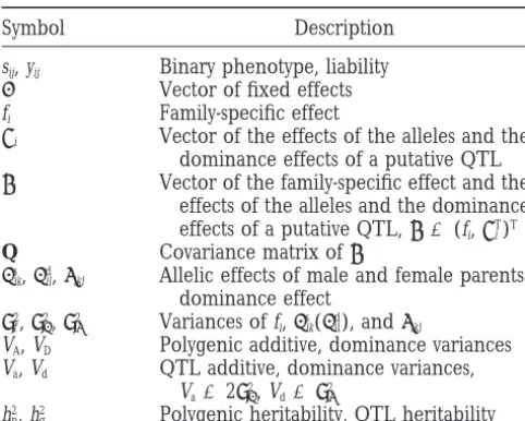
, Description of symbols used in the text domin

where zaij 5(zsij1, 12zsij1, zdij1, 12 zdij1)T, zdij 5(zsij1zdij1, zsij1

Symbol Description

(12zd

ij1), (12zsij1)zdij1, (12zsij1)(12zdij1))T, sij, yij Binary phenotype, liability

b Vector of fixed effects

fi Family-specific effect

hi Vector of the effects of the alleles and the dominance effects of a putative QTL

gi Vector of the family-specific effect and the

Var(zaij)5

1

ps

ij1(12psij1) 2psij1(12psij1)

2ps

ij1(12psij1) psij1(12psij1)

0 0

0 0

0 0

0 0

pd

ij1(12pdij1) 2pdij1(12pdij1)

2pd

ij1(12pdij1) pdij1(12pdij1)

2

, effects of the alleles and the dominance

effects of a putative QTL,gi5(fi,hTi)T

Q Covariance matrix ofgi

as

ik,adil,dikl Allelic effects of male and female parents,

dominance effect

s2

f,s2a,s2d Variances of fi,asik(adil), anddikl

VA, VD Polygenic additive, dominance variances

Va, Vd QTL additive, dominance variances,

Va52s2a, Vd5 s2d

Cov(zaij,zdij)5

1

ps

ij1(12psij1)pdij1 pij1s(12psij1)(12pdij1)

2ps

ij1(12psij1)pdij1 2pij1s(12psij1)(12pdij1) pd

ij1(12pdij1)psij1 2pdij1(12pdij1)psij1

2pd

ij1(12pdij1)psij1 pdij1(12pdij1)psij1 h2_{p, h}2

q Polygenic heritability, QTL heritability

is further standardized by settings2

ε 51 and t50

(Har-villeand Mee 1984; McCulloch 1994; Sorensen et al. 1995). Under the “standardized threshold model,”

2ps

ij1(12psij1)pdij1 2pij1s(12psij1)(12pdij1) ps

ij1(12psij1)pdij1 pij1s(12psij1)(12pdij1) pd

ij1(12pdij1)(12psij1) 2pdij1(12pdij1)(12psij1)

2pd

ij1(12pdij1)(12psij1) pdij1(12pdij1)(12psij1)

2

the vectors of fixed and random effects,bandgi,

corre-spond to s21

ε b and s2ε1gi, respectively (Harville and

Mee1984). In subsequent discussion, we use the stan-dardized threshold model.

If the putative QTL is not at a marker locus or even

if the QTL is at the marker locus but the marker is not Var(zdij)5

1

ps

ij1pdij1(12psij1pdij1) 2(ps

ij1)2pdij1(12pdij1) 2(pd

ij1)2psij1(12psij1) 2ps

ij1pdij1(12psij1)(12pdij1)

fully informative, the genotype of the QTL is unobserv-able so that zijare missing. We can only infer the

distribu-tion of zij from observed genotypes of linked markers.

2(ps

ij1)2pdij1(12pdij1)

Define the probabilities of zs

ij151 and zdij151

condi-tional on marker information by ps

ij15Pr(zsij151|IM) _ps

ij1(12pdij1)[12psij1(12pdij1)]

and pd

ij15Pr(zdij15 1|IM), respectively. Let E(zij|IM) be the

2ps

ij1pdij1(12psij1)(12pdij1)

conditional expectation of zijgiven marker information

(IM). The linear model (1) can be approximated by the 2_ps

ij1(12psij1)(12pdij1)2

following heterogeneous residual variance model:

2(pd

ij1)2psij1(12psij1)

yij5xTijb 1fi 1E(zij|IM)Thi1eij. (2)

2ps

ij1pdij1(12psij1)(12pdij1)

The residual variance is

pd

ij1(12psij1)[12pdij1(12psij1)]

Var(eij)5Var(yij|IM,b, fi,hi)

2pd

ij1(12pdij1)

5 hT

iVar(zij|IM)hi 1 s2ε5 Vij,

wheres2

ε 51 (as chosen in the standardized threshold model) andhT

iVar(zij)hi is the variance not explained

2ps

ij1pdij1(12psij1)(12pdij1) 2ps

ij1(12psij1)(12pdij1)2 2pd

ij1(12pdij1)(12psij1)2

(12ps

ij1)(12pdij1)[12(12psij1)(12pdij1)]

2

.

due to the uncertainty of the QTL genotype (Xu1996b, 1998). Given conditional probabilities pS

ij1and pdij1, the

expectation and variance matrices ofxij are

The conditional probabilities, ps

ij1 and pdij1, are

calcu-E(zij|IM)5(psij1, 12psij1, pdij1, 12pdij1,

lated using the simplified multipoint method proposed ps

ij1pdij1, psij1(12 pdij1), (12psij1)pdij1, in four-way crosses (Rao and Xu 1998). The method

requires known marker linkage phases in the parents. (12ps

ij1) (12pdij1))T

the offspring. If grandparents are also genotyped, the f(S,g|b,Q)5g(S|g,b)p(g|Q). linkage phases can be accurately reconstructed;

other-The EM-algorithm starts from the joint log-likelihood wise, a relatively large number of offspring for each

function of the complete data family is required (Knottet al. 1996). When family sizes

are too small to provide reasonable accuracy of linkage _L5 log f(S,g|b,Q) phase inference, alternative models, e.g., the

identical-5

o

n

i51

o

ni

j51

[sijlog Pij 1(12 sij)log(12 Pij)]

by-descent (IBD)-based random model approach, should be considered, which are discussed later.

Maximum-likelihood estimation of genetic variances: ₁

_o

n

i51

logp(gi|Q). (4)

A maximum-likelihood (ML) method is proposed for estimation of the variance components. We first obtain

In the (m1 1)th cycle of iteration, the E-step consists the sample density, g(sij|gi,b), using the probit

relation-of computing ship between the binary phenotype and the model

ef-fects _M(Q|Q(m)₎5_E{log(f(S,g|b,Q)|_S,Q(m)_)},

g(sij|gi,b)5 [Pr(yij. 0|gi,b)]Sij[12 Pr(yij .0|gi,b)]12sij the conditional expectation of the log-likelihood of the

complete data given the estimated parameters Q(m)_from

5

3

F

1

mij

√

Vij

24

sij

3

12 F

1

mij

√

Vij

24

12sij

, the previous cycle of iteration. In the M-step M(Q|Q(m)₎

has to be maximized with respect to Q. Differentiation with respect tos2

f,sa2, ands2d, setting derivatives to zero,

whereF(·) is the standardized normal distribution

func-and solving for s2

f,s2a, ands2d yield the following

up-tion andmij 5xTijb 1fi1 E(zij|IM)Thi. For notational

sim-dates: plicity, we denote Pij 5Pr(yij. 0|gi,b)5 F(mij/

√

Vij) in

subsequent discussion. Conditional ongi5 (fi,hTi)T,

in-s2(m11)

f 5

1 n

o

n

i51 E(f2

i|S,Q(m))

dividuals within the same family are independent. Hence, the joint density for the ith family is

5 1

n

o

n

i51

[Var(fi|S,Qm))1 E2(fi|S,Q(m))],

p

ni

j51

g(sij|gi,b)5

p

ni

j51 Psij

ij(12 Pij)12sij.

s2(m11)

a 5 1

4n

o

2

k51

o

n

i51

[E((as

ik)2|S,Q(m))1E((adik)2|S,Q(m))]

For n independent families, the overall joint density is

g(S|g,b)5

p

n

i51

p

ni

j51

g(sij|gi,b)5

p

n

i51

p

ni

j51 Psij

ij(1 2Pij)12sij,

5 1

4n

o

2

k51

o

n

i51

[Var(as

ik|S,Q(m))1E2(asik|S,Q(m))

whereg 5(gT

1 gT2 · · ·gTn)Tand S5(s11s12· · · snnn)T. The ₁

Var(ad

ik|S,Q(m))1E2(adik|S,Q(m))],

likelihood function is obtained by integrating out the random effects g and thus becomes a function of the

s2(m11)

d 5 1

4n

o

2

k51

o

2

l51

o

n

i51

E((dikl)2|S,Q(m))

data S and the parametersj 5(bTs2

f s2a s2d)T. The

log-likelihood function has the form of

5 1

4n

o

2

k51

o

2

l51

o

n

i51

[Var(dikl|S,Q(m))1E2(dikl|S,Q(m))].

l(j|S)5 log

#

g(S|g,b)p(g|Q)dg, (3) where Q 5diag(s2

f s2as2as2as2as2ds2dsd2s2d), as previ- Although the algorithm is conceptually

straightfor-ously defined, ward, it is difficult to carry out the updates exactly be-cause the posterior means

p(g|Q)5

p

n

i51

p(gi|Q),

{E(fi|S,Q(m)), E(asik|S,Q(m)), E(adil|S,Q(m)),

E(dikl|S,Q(m))}

and

and the posterior variances

p(gi|Q)5(2p)22|Q|21/2exp{21/2gTiQ21gi}.

{Var(fi|S,Q(m)), Var(asik|S,Q(m)),

Other types of distribution, rather than normal, may be

specified for gi. The maximum-likelihood estimation _Var(ad

il|S,Q(m)), Var(dikl|S,Q(m))}

(MLE) ofjis obtained by maximizing the marginal log

likelihood l(j|S) (Searle et al. 1992; Fahrmeir and do not have explicit expressions. In principle, the poste-rior means and variances can be obtained via numerical Tutz1994).

Direct maximization of (3) is cumbersome due to the integration or a Monte Carlo method (e.g.,Fahrmeir and Tutz 1994; McCulloch 1994; Chan and Kuk high-dimensional integral structure. Instead, we may

and thus are not feasible for whole-genome scanning

for QTL. To ease the computational burden, analytic Vˆd5

1

s´2

f

12 sˆ2

f

11

2

sˆ2

d. (5)

approximations of the posterior means and the

poste-rior variances are needed. In this study, the posteposte-rior _{The estimated proportions of variances explained by} means are approximated by the posterior modes fˆi, aˆsik, _{the polygene and the QTL are}

aˆd

il, anddˆikl(i51, · · ·, n; k, l51, 2) and the posterior

variances by the posterior curvatures Vˆf

i, Vˆsik, Vˆdil, and

hˆ2 p5

Vˆ_A VˆA1Vˆa1Vd11

and hˆ2 q5

Vˆ_a VˆA1Vˆa1Vd11

, Vˆdikl(i5 1, · · ·, n; k, l5 1, 2). Both the posterior

modes and posterior curvatures are obtained by using

respectively. a Fisher-scoring algorithm, which is described in the

Tests of hypotheses: Although the additive and domi-appendix.

nance effects can be tested individually, we investigate The resulting EM-algorithm with the Fisher-scoring

only the overall test of the presence of QTL. The null algorithm embedded in each E-step jointly estimates

hypothesis is H0:sa2 5 s2d50. The alternative

hypothe-b,g,s2

f,s2a, ands2das follows:

sis is H1:s2a?0 ors2d? 0. The likelihood-ratio test

sta-1. Choose starting valuess2(0)

f ,s2(0)a , ands2(0)d . tistic is used to test the presence of QTL, which is defined

2. Compute posterior mode estimates fˆi,aˆsik,aˆdil, anddˆikl _as

(i5 1, · · ·, n; k, l 5 1, 2) and posterior curvature

L 5 22(L02L1), (6)

estimates Vˆf

i, Vˆsik, Vˆdil and Vˆdikl(i5 1, · · ·, n; k, l5 1,

2) via the Fisher-scoring algorithm with variance

where L1is the log likelihood evaluated under the

alter-components replaced by their current estimates

native hypothesis (full model) and L0is that evaluated

s2(m)

f ,s2(m)a , ands2(m)d . The estimated fixed effectbˆ, is

under the null hypothesis (reduced model). also obtained in this step.

Although the EM-algorithm with the Fisher-scoring 3. EM-step: Computes2(m11)

f ,s2(ma 11), ands2(md 11)by

embedded in each E-step has eliminated the necessity of numerical integration and provides a convenient way

s2(m11)

f 5

1 n

o

n

i51

[Vˆf(m)

i 1 (fˆ(m)i )2],

for estimation of variance components, it does not auto-matically generate the numerical value of the likelihood. To calculate the likelihood value, one still needs

numeri-s2(m11)

a 5 1

4n

o

2

k51

o

n

i51

[Vˆs(m)

ik 1 (aˆs(m)ik )21Vˆd(m)ik

cal integration. Fortunately, it is manageable in this stage because the parameters are replaced by their MLEs

1(aˆd(m)

ik )2],

without updating. The Monte Carlo numerical integra-tion is applied here due to the high dimensionality of

s2(m11)

d 5 1

4n

o

2

k51

o

2

l51

o

n

i51

[Vˆd(m)

ikl 1(dˆ(m)ikl)2].

the random effects. The log-likelihood value under the alternative model evaluated at the MLE is

4. If convergence is reached, set sˆ2

f 5 s2(mf 11),sˆ2a5

s2(m11)

a , and sˆ2d5 s2(md 11); otherwise, increase m by 1

L15

o

n

i51

log

#p

ni

j51

g(sij|gi,bˆ)p(gi|Qˆ )dgi.

and return to step 1.

Note that under the standardized threshold model, _{The Monte Carlo approximation of}

#p

ni

j51 g(sij|gi,bˆ)

s2

f,s2a, ands2dare actually ratios of variance components. _p

(gi|Qˆ )dgiis obtained by

Recall that the value of the residual variance has been set to unity, which leads the above variances to be

#p

ni

j51

g(sij|gi,bˆ)p(gi|Qˆ )dgi≈

1

M

o

M

k51

p

ni

j51

g(sij|g(k)i ,bˆ),

s2

f 5(s2ε)21(1⁄2VA1 1⁄4VD1VC),

whereg(k)

i for k5 1, · · · , M is a random sample

simu-wheres2

ε 51⁄2VA1 3⁄4VD11 as given earlier. Let us

as-lated from distributionp(gi|Qˆ ), and M is the length of

sume that VD5VC50 so that we have the relationships

the Monte Carlo simulation. The Monte Carlo approxi-mation becomes sufficiently accurate when M is very

s2

f 5

1_⁄ 2VA 1_⁄

2VA11

, s2

a5

1_⁄ 2Va 1_⁄

2VA1 1

, s2

d5₁ Vd

⁄2VA1 1

,

large. The empirical value of M 5 5000 (Xu and Atchley1996b) is adopted in this study.

where VA, Va, and Vdare additive variance of the polygene _{Under the null hypothesis, model (2) has been}

re-and additive re-and dominance variances of the QTL, re- _{duced to} spectively. These genetic variances are obtained by

us-ingsˆ2

f,sˆ2a, andsˆ2dand solving for the above equations: yij5xTijb 1 fi1εij,

where fizN(0,s2f) andεijzN(0, 1). The log-likelihood

VˆA5

2sˆ2

f

12 sˆ2

f

, Vˆa5 2

1

sˆ2

f

12 sˆ2

f

11

2

sˆ2

a,

h2

q5 0.10 (VA5 0.80, Va5 0.10, Vd50.10), L05

o

n

i51

log

#p

ni

j51

g(sij|fi,bˆˆ)p(fi|sˆˆ2f)dfi,

h2

q5 0.25 (VA5 0.50, Va5 0.25, Vd50.25),

wherebˆˆ andsˆˆ2

f are the MLE under H0. _h2

q5 0.40 (VA5 0.20, Va50.40, Vd50.40);

There is a numerical problem with the Monte Carlo

approximation; that is, when the family size becomes (2) sampling strategy (number of families3family size): large,

p

nij51 g(sij|g(k)i ,bˆ) tends to be close to zero, causing 2 3 250, 5 3 100, 10 3 50, 15 3 33, 20 3 25, and

computational underflows. This can be circumvented 50310; (3) marker polymorphism: two, four, and eight

by first calculating equally frequent alleles at each marker.

Instead of performing simulations under all possible combinations of parametric settings, we simulated a situ-C(i,k)5

o

ni

j51

log g(sij|g(k)i ,bˆˆ)5

1 M

o

M

k951

o

ni

j51

log g(sij|g(ki9),bˆ)

ation in which the central level is chosen for each factor considered above. We referred to this as the “standard and then taking

setting,” which is described as follows: h2

q 5 0.25, 10

families each with 50 sibs and four alleles per marker. log

3

1

M

o

M

k51

p

ni

j51

g(sij|g(k)i ,bˆ)

4

When the influence of different levels of a factor on the performance of the method is examined, all other factors are set to the standard levels.

5 log

3

1 M

o

M

k51

eC(i,k)1 1

M

o

M

k51

o

ni

j51

log g(sij|g(k)i ,bˆ)

4

.

The simulations were repeated 100 times for each parametric setting. The standard error of the parameter Therefore, the Monte Carlo-evaluated log-likelihood

estimate was calculated from the standard deviation of function under the alternative hypothesis is

the estimates among the 100 replicates. To estimate the statistical power, we ran 1000 additional replicates with L15

o

n

i51

log

3

1 M

o

M

k51

eC(i,k)1 1

M

o

M

k51

o

ni

n51

log g(sij|g(k)i ,bˆ)

4

.

no QTL segregating while the other two factors were set at their standard levels. We augmented the polygenic The Monte Carlo log-likelihood function under the null _{variance such that the total genetic variance of the} liabil-hypothesis L0 is similarly calculated. _{ity remained unchanged. The statistical power was}

deter-mined by counting the (proportion) number of runs (over the 100 replicates) that have test statistics greater

SIMULATION STUDIES _{than a chromosome-wise empirical critical value. The}

empirical critical value was obtained by choosing the Experimental design: Application of the proposed

95th and 99th percentiles of the highest test statistic method is illustrated via Monte Carlo simulation

experi-over the 1000 runs under the null model (no QTL ments. The following properties were examined: the

segregating). bias, the standard error of parameter estimation, and

Under the standard setting, results of the proposed the statistical power of QTL detection. We simulated a

GLMM approach were then compared with those of the single chromosome segment of length 80 cM with nine

simple LMM analysis, where the binary data were treated evenly spaced codominant markers. In most cases, four

as if they were continuous. We modified the random equally frequent alleles were simulated at each marker

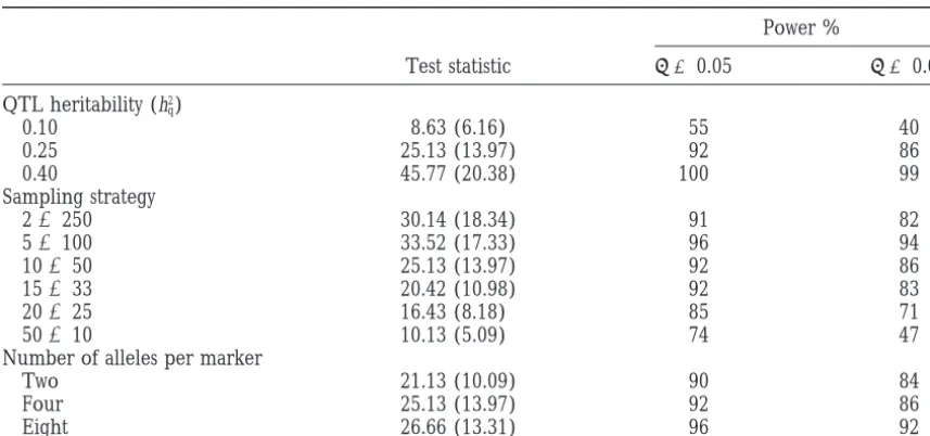
locus. A single QTL residing at position 25 cM and 12 model method ofXu (1998) so that it can be applied to the populations that were used in this study. additional independent loci of equal effect (called the

polygene) were simulated for the liability. The domi- Results: The empirical critical values at type I error rates of 0.05 and 0.01 obtained from 1000 replicated nance effect of the polygene was assumed to be absent.

Both the allelic effects and the allelic interaction effects simulations were 7.87 and 10.73, respectively. The aver-age likelihood-ratio test statistics and the power esti-(dominance) of the QTL were assumed to be normally

distributed and so was the polygenic effect. Value of the mates over 100 replicated simulations are summarized in Table 2. As expected, the average test statistic in-liability of each individual took the sum of an overall

mean, values of QTL additive and dominance effects, creases as the QTL heritability increases. The statistical power also shows the same trend. The sampling strategy polygenic effect, and a residual error sampled from a

standardized normal distribution. The observable bi- also has an effect on the test statistic and the power. When the total number of individuals is fixed, the aver-nary phenotype was set to be 1 if corresponding liability

exceeded 0, and 0 otherwise. The fixed effect contained age test statistic increases as the family size increases. However, when the number of families is too small, e.g., the population mean of the liability only, which led to

a proportion of the trait presence (incidence) of 40%. two, the average test statistic tends to decrease, primarily due to sampling error of the parents. There is an optimal To examine the effect of different factors on the

per-formance of the method, we varied each of the following sampling strategy, any deviation from which will cause a decrease in the test statistic and the power. Marker factors successively: (1) the proportion of variance

TABLE 2

Average test statistics and empirical powers of QTL detection obtained from 100 replicated simulations

Power %

Test statistic a 50.05 a 50.01

QTL heritability (h2_q)

0.10 8.63 (6.16) 55 40

0.25 25.13 (13.97) 92 86

0.40 45.77 (20.38) 100 99

Sampling strategy

23250 30.14 (18.34) 91 82

53100 33.52 (17.33) 96 94

10350 25.13 (13.97) 92 86

15333 20.42 (10.98) 92 83

20325 16.43 (8.18) 85 71

50310 10.13 (5.09) 74 47

Number of alleles per marker

Two 21.13 (10.09) 90 84

Four 25.13 (13.97) 92 86

Eight 26.66 (13.31) 96 92

The standard errors of test statistics are given in parentheses.

power. The average test statistic and the statistical power observed in the estimates of variance components. The bias caused by the first approximation can be reduced increase as marker polymorphism increases.

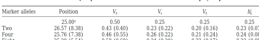
The properties of the method were investigated un- by increasing marker density and allelic polymorphism because the uncertainty of the QTL genotype inference der three levels of proportion of variance explained by

the QTL while the other factors were set at their stan- can be reduced so that the single normal distribution adequately approximates the mixed distribution. The dard levels (see Table 3). As expected, the estimate of

position of the QTL is quite accurate when h2

qis not too bias caused by the second approximation can be

pre-vented by using a sampling-based Markov chain Monte low. A bias toward the center of the chromosome

seg-ment was observed when h2

q50.10. The estimation er- Carlo (MCMC) algorithm, which is discussed in the next

section. Because most QTL may be in the range of ror of the QTL position was also large when h2

qis small.

Both the polygenic variance and the variances of QTL medium to small in size (variance) and the bias is slight when the true QTL heritability is in this range, the bias effects were underestimated by the method. The

under-estimation can be severe when the true variances are should not be of major concern for this method. The sampling strategy was investigated with the other high. There are two approximations in the derivation

of the method, one being the mixture of four normal factors set at their standards (see Table 4). The estimate of the QTL position is unbiased when family size is distributions of the residual of the liability

approxi-mated by a single normal distribution with heteroge- not too small, but larger estimation errors are observed when either too few or too many families are used. The neous variance and the other being the posterior means

and variances replaced by the posterior modes and cur- bias in the estimates of variance components also seems to follow the same trend—the least bias at the optimal vatures. These two approximations may explain the bias

TABLE 3

Mean estimates of QTL parameters under different levels of QTL heritability

QTL heritability Position VA Va Vd h2q

0.10 True 25 0.80 0.10 0.10 0.10

Estimate 29.80 (16.50) 0.71 (0.60) 0.13 (0.12) 0.08 (0.10) 0.10 (0.05)

0.25 True 25 0.50 0.25 0.25 0.25

Estimate 25.76 (7.38) 0.46 (0.55) 0.26 (0.10) 0.21 (0.24) 0.24 (0.08)

0.40 True 25 0.20 0.40 0.40 0.40

Estimate 24.68 (3.27) 0.29 (0.45) 0.32 (0.27) 0.32 (0.24) 0.33 (0.09)

TABLE 4

Mean estimates of QTL parameters under different sampling strategies (number of families3family size)

Sampling strategy Position VA Va Vd h2q

25.00a _{0.50 0.25 0.25 0.25}

23250 25.75 (9.27) 0.42 (0.60) 0.21 (0.24) 0.21 (0.26) 0.23 (0.09)

53100 25.23 (5.03) 0.49 (0.53) 0.25 (0.23) 0.23 (0.19) 0.25 (0.09)

10350 25.76 (7.38) 0.46 (0.50) 0.26 (0.22) 0.21 (0.24) 0.24 (0.08)

15333 25.62 (10.08) 0.42 (0.43) 0.21 (0.17) 0.19 (0.15) 0.22 (0.08)

20325 25.02 (7.34) 0.51 (0.41) 0.23 (0.19) 0.18 (0.13) 0.21 (0.07)

50310 27.14 (15.86) 0.49 (0.36) 0.19 (0.13) 0.17 (0.10) 0.20 (0.06)

The standard errors of estimates obtained by the standard deviation of 100 replicated simulations are given in parentheses.

a_{Numbers in this row are the true parametric values.}

sampling strategy (53 100). The estimation errors of for binary traits but to illustrate that the proposed method behaves like the existing QTL mapping proce-the variance components, however, seem to decrease

monotonically as the number of families increases. dures developed for regular quantitative traits. The con-clusion is that the method behaves as expected and Increasing the level of marker polymorphism can

im-prove the estimate of QTL position but has limited effect works well in the situations examined. on the estimation of the variance components (Table 5).

The empirical critical values at type I error rates of

DISCUSSION

0.05 and 0.01 obtained from 1000 replicated simulations

were 8.01 and 14.61, respectively, when treating binary Both the random model approach of QTL mapping for normally distributed traits and the fixed model ap-data as normally distributed. In the “standard setting,”

the power estimates over 100 replicated simulations proach of QTL mapping for binary traits are well devel-oped (FulkerandCardon1994;HackettandWeller were 83 and 60%, respectively, lower than 92 and 86%,

which were observed under the threshold model. The 1995; Xu and Atchley 1995; Grignola et al. 1996; Visscheret al. 1996;Xu1996a;XuandAtchley1996a; estimates of the QTL position and its standard error

were 25.52 and 11.75, respectively. The heritability esti- Rebai1997;RaoandXu1998). Our contribution is to develop the random model approach of QTL mapping mate of the observed binary trait and its standard error

were 0.16 and 0.078, respectively. We converted the for binary data, which is a combination of the two exist-ing approaches. Although neither approach is compli-heritability estimate of the observed binary trait into

that of the liability (Lynch andWalsh 1998, p. 743) cated enough by itself to prevent the use of an exact ML method, the combination becomes cumbersome and obtained the liability heritability estimate 0.28 and

it standard error 0.14. As expected, the proposed enough that there does not exist an exact form of ML method due to the lack of analytically and computation-method has a higher statistical power and also produces

more accurate estimates of the QTL position and the ally tractable mixing distributions. The method pre-sented here illustrates the use of a GLMM for QTL heritability than the method that directly analyzes the

binary trait. mapping with some approximations (see simulation

studies for the approximations). Results of Monte The purpose of the simulation experiments is not to

exhaustively search for the best design of QTL mapping Carlo simulations show that the approximations are well

TABLE 5

Mean estimates of QTL parameters under different levels of marker polymorphism

Marker alleles Position VA Va Vd h2q

25.00a _{0.50 0.25 0.25 0.25}

Two 26.57 (8.38) 0.43 (0.40) 0.23 (0.22) 0.20 (0.16) 0.23 (0.07)

Four 25.76 (7.38) 0.46 (0.55) 0.26 (0.22) 0.21 (0.24) 0.24 (0.08)

Eight 25.20 (5.54) 0.58 (0.60) 0.24 (0.20) 0.22 (0.17) 0.23 (0.08)

The standard errors of estimates obtained by the standard deviation of 100 replicated simulations are given in parentheses.

justified because both the location and the effects of the the sample of offspring within the single family to ensure that segregation of the QTL alleles in the parents is simulated QTL are well estimated by the approximate

method. These minor assumptions have yielded a com- detectable. The method is heavily dependent on the parents sampled. If the parents do not segregate at a putationally attractive ML method. With this

approxi-mate ML, we can perform genome scanning of QTL QTL, there is no power to detect it even though the QTL segregates in the population in which these two for binary traits, just as we do for regular quantitative

traits. To the best of our knowledge, this is the first parents are sampled. One can combine information from multiple families to ensure that segregating par-attempt to map QTL for binary data using an approach

that is consistent with classical quantitative genetic ents are sampled (Muranty1996;Xie et al. 1998;Xu 1998). There are two strategies for combining data from theory.

Approximations occurred twice in the derivation of multiple families: the fixed model and the random model approaches. Which model should we choose? the method, one being that the mixture of four normal

distributions of the residual in the scale of liability is One should decide whether the parents chosen to form the mapping population are a random sample from a approximated by a single normal distribution and the

other being that the posterior means and posterior vari- hypothetical large population (base population). If they are, one should consider the use of the random model ances are replaced by the posterior modes and

curva-tures. The first approximation can be easily relaxed; i.e., approach, provided that one is interested in understand-ing the genetic properties of the base population. If the we can directly use the mixed distribution rather than

a single distribution, although the exact expression of parents of the mapping population are not randomly sampled and one has no desire to understand the base the Fisher-scoring algorithm is not as clean as it is now.

Analytically, the second approximation can also be re- population, but only the mapping population, then the fixed model is more appropriate. Under the random laxed, but the price is an unrealistic computational time.

The posterior means and posterior variances can be model approach, we are interested in making a statistical inference about the base population. Namely, the esti-calculated via a sampling-based approach, e.g., the Gibbs

sampler. The combination of the EM with the sampling- mated QTL variances may reflect the actual genetic variation existing in the population where the experi-based approaches is called the Monte Carlo EM

(Fahr-meirandTutz1994;McCulloch1994;ChanandKuk mental units are sampled.

Interestingly, we can use the fixed model approach 1997). The Monte Carlo EM is feasible for evaluation

of a single point of a genome but unrealistic for the to solve the random model problem. In this situation, we have a random model in our mind; i.e., we are inter-whole genome scanning because many points need to

be evaluated. At any single point, there are many EM- ested in inferring the statistic(s) drawn from the sample to the base population, but we may first estimate and steps, each requiring many cycles of the Gibbs sampler

(Gibbs chain). If the Gibbs chain is long, the time re- test the first moment statistics (the effects) as if they were fixed effects and then calculate the variance of the quired in the total genome scanning can be unrealistic.

If the chain is too short, on the other hand, the posterior effects by relaxing the fixed assumption. Statistically, this approach is identical to Henderson’s method III means and posterior variances will deviate from the

exact values. At this point, the approximate ML method for variance component estimation (Searleet al. 1992). Because the model is a random model, but the statistical is perhaps better suited than the Monte Carlo EM.

An-other exact method is the Bayesian approach of QTL method itself is not a real random model approach, we call it the pseudorandom model approach. This ap-mapping. Instead of performing whole-genome

scan-ning, one can treat the positions of multiple QTL as proach has been previously examined in QTL mapping using multiple families of line crosses (Xu 1998) and unknown variables. The number of QTL can even be

treated as an unknown variable and be searched simulta- outbred populations (Knott et al. 1996). Yi and Xu (1999) recently developed the pseudorandom model neously (Heath 1997; Uimari and Hoeschele 1997;

Sillanpaa and Arjas 1998). The full Bayesian treat- approach of QTL mapping for binary data using multi-ple families. We showed that the pseudorandom model ment must also be implemented via the sampling-based

approach, which is of course time consuming. The full approach is quite efficient and computationally much faster than the true random model approach. There is, Bayesian treatment may show some advantages over the

ML approach, but the price is the increased computa- though, a complication in the interpretation of the test statistic in the pseudorandom model. Because the QTL tional burden and a reduced intuitiveness of the

ge-nome scanning. Although the full Bayesian approach effects are tested and the number of QTL effects in-creases as the number of families inin-creases, the critical seems to be the direction of QTL mapping research in

the future (Satagopanet al. 1996;Heath1997;Uimari value of the test statistic used to declare statistical sig-nificance changes accordingly as the number of families andHoeschele 1997;Sillanpaa and Arjas 1998), it

cannot replace the existing ML approach in practice. changes. This is undesirable because the guidelines for significance declaration suggested by Lander and Conventional QTL mapping procedures utilize a

model approach developed in this study does not have and reconstruct a full-rankedPiwith a reduced

dimen-sion. The principle of the IBD-based method is not that drawback and is statistically more sound. It should

complicated, but implementation of the method de-complement, but not replace, the existing

pseudoran-serves further investigation. dom model approach.

In this study, we have assumed that QTL effects are The QTL mapping procedure presented in this study

normally distributed. In reality, the number of alleles is based on known marker linkage phases in the parents.

and the allelic frequencies of a putative QTL in the base Therefore, the inference of marker linkage phases is a

population are rarely known, nor are the distributions prerequisite of the method. There are several ways to

of the effects of the QTL. However, drawing inferences deduce the parental haplotypes in outbred populations:

about the QTL variance via the normal distribution is (1) track alleles from the parental genotype through the

a natural way to characterize genetic variation in the segregating progeny population; (2) use grandparental

base population. In addition, normal distribution of the genotypes; or (3) genotype the parents directly using

allelic effects is usually a very robust assumption. This PCR-based marker technology from parental gametes

has been verified for normal traits byXuandAtchley (Williams1998). The accuracy of phase inference

us-(1995), who found that, for data simulated under a ing method (1) largely depends on the family size. When

biallelic model, the analysis based on the normal distri-the family size is small, inference of distri-the parental linkage

bution provided very accurate estimates of QTL vari-phases is subject to error, which will likely reduce the

ances. power of QTL detection. Therefore, the method

pre-Although we demonstrate the statistical method of sented is practical only for species with large family sizes,

QTL mapping using full-sib families as an example, in say ni$ 20 for i5 1, . . . , n. To apply this method to

principle, families from other types of mating designs QTL mapping in species with small family sizes, e.g.,

can be readily incorporated by modifying model (2) human and some other mammals, we must modify the

and the conditional probabilities ps

ij1and pdij1. The model

method by incorporating the IBD approach (Fulker

considered here assumes only one QTL on the chromo-andCardon1994). The IBD-based approach requires

some. In reality, complex binary traits may be controlled only the proportion of allelic sharing by two relatives

by multiple loci. With our random model approach, (e.g., sibs) and does not distinguish as to which alleles

QTL located on other chromosomes will be absorbed of the parents are being shared by the sibs. This

elimi-into the polygenic term. If there are multiple QTL in nates the necessity of linkage phase information.

Incor-the same chromosome, Incor-the estimation tends to be biased poration of the IBD-based approach into the current

because of interference caused by QTL located on the method is straightforward; one simply replaces the

ge-same chromosome but outside the tested region. This netic (random) effects of the parents by the genetic

problem can be solved by resorting to the concept of effects of the progenies and solves for the genetic effects

composite interval mapping (Jansen1994;Zeng1994). of the progenies in the Fisher-scoring step with Q

re-Our model can be readily extended to implement com-placed by

posite interval mapping by incorporating markers on other chromosome regions as covariates. These con-trolled marker effects can be equally treated as random Qi 5

1

s2

f

0 0

Pis2a

2

5

1

s2

f 0 ··· 0

0 p11s2a ··· p1nis2a

A A ··· A

0 p1nis2a ··· pninis2a

2

,

effects and their variances can absorb QTL variances outside the tested region so that bias can be reduced or eliminated (XuandAtchley1995).

wheres2

f is the variance of family-specific effects as

de-We thank Dr. Bruce Walsh and an anonymous reviewer for their

fined earlier,s2

ais proportional to the additive genetic critical comments on an earlier version of the manuscript. We also

variance of the QTL, and Pi is an ni 3 ni IBD matrix thank Dr. Damian Gessler for his helpful comments on the manu-script. This research was supported by the National Institutes of Health

with the jj9elementpjj9defined as the IBD proportion

Grant GM55321-01 and the U.S. Department of Agriculture National

shared by sibs j and j9at the QTL. Note that dominance

Research Initiative Competitive Grants Program 97-35205-5075.

and other effects are assumed absent. The vector of random effects is now defined asgi5 (fi gi1· · · gini)T,

where gijis the additive genetic effect of the QTL of the _{LITERATURE CITED}

jth sib in the ith family. The IBD matrix at the QTL is

Almasy, L.,andJ. Blangero, 1998 Multipoint quantitative-trait

link-unobservable but can be estimated from the IBD matri- _{age analysis in general pedigrees. Am. J. Hum. Genet. 62: 1198–} ces of linked markers using the multipoint method 1211.

Chan, J. S. K.,andA. C. Kuk, 1997 Maximum likelihood estimation

(KruglyakandLander1995;AlmasyandBlangero

for probit-linear mixed models with correlated random effects.

1998). The problem with the IBD-based method is that _{Biometrics 88: 86–97.}

one needs to invert the matrix Qi, which further requires Fahrmeir, L., and G. Tutz, 1994 Multivariate Statistical Modeling

Based on Generalized Linear Models. Springer-Verlag, New York. inverting matrix Pi. However, in most situations Pi is

Falconer, D. S.,andT. F. C. Mackay, 1996 Introduction to Quantita-not invertable (Quantita-not of full rank). Numerically, one must _{tive Genetics, Ed. 4. Longman, London.}

Fulker, D. W., and L. R. Cardon, 1994 A sib-pair approach to

interval mapping of quantitative trait loci. Am. J. Hum. Genet. Xie, C., D. D. G. GesslerandS. Xu, 1998 Combining different line crosses for mapping quantitative trait loci using the IBD-based

54:1092–1103.

Goldgar, D. E., 1990 Multipoint analysis of human quantitative variance component method. Genetics 149: 1139–1146. Xu, S., 1996a Computation of the full likelihood function for esti-genetic variation. Am. J. Hum. Genet. 47: 957–967.

Grignola, F. E., I. HoescheleandB. Tier, 1996 Mapping quantita- mating variance at a quantitative trait locus. Genetics 144: 1951– 1960.

tive trait loci via residual maximum likelihood. I. Methodology.

Genet. Sel. Evol. 28: 479–490. Xu, S., 1996b Mapping quantitative trait loci using four-way crosses. Genet. Res. 68: 175–181.

Haley, C. S.,andS. A. Knott, 1992 A simple regression method

for mapping quantitative trait loci in line crosses using flanking Xu, S., 1998 Mapping quantitative trait loci using multiple families of line crosses. Genetics 148: 517–524.

markers. Heredity 69: 315–324.

Haseman, J. K.,andR. C. Elston, 1972 The investigation of linkage Xu, S.,andW. R. Atchley, 1995 A random model approach to interval mapping of quantitative trait loci. Genetics 141: 1189– between a quantitative trait and a marker locus. Behav. Genet.

2:3–19. 1197.

Xu, S.,andW. R. Atchley, 1996a Mapping quantitative trait loci Hackett, C. A.,andJ. I. Weller, 1995 Genetic mapping of

quantita-tive trait loci for traits with ordinal distributions. Biometrics 51: for complex binary diseases using line crosses. Genetics 143: 1417–1424.

1252–1263.

Harville, D. A.,andR. W. Mee, 1984 A mixed-model procedure Xu, S., andW. R. Atchley, 1996b A Monte-Carlo algorithm for maximum likelihood estimation of variance components. Genet. for analyzing ordered categorical data. Biometrics 40: 393–408.

Heath, S. C., 1997 Markov chain Monte Carlo segregation and Sel. Evol. 28: 329–343.

Yi, N.,andS. Xu, 1999 Mapping quantitative trait loci for complex linkage analysis of oligogenic models. Am. J. Hum. Genet. 61:

784–760. binary traits in outbred populations. Heredity 82: 668–676. Zeng, Z. B.,1994 Precision mapping of quantitative trait loci. Genet-Jansen, R. C., 1993 Interval mapping of multiple quantitative trait

loci. Genetics 135: 205–211. ics 136: 1457–1468. Jansen, R. C., 1994 Controlling the type I and type II errors in

Communicating editor:T. F. C. Mackay mapping quantitative trait loci. Genetics 138: 871–881.

Knott, S. A., J. M. ElsenandC. S. Haley, 1996 Methods for multi-ple-marker mapping of quantitative trait loci in half-sib popula-tions. Theor. Appl. Genet. 93: 71–80.

Kruglyak, E. S.,andE. S. Lander, 1995 Complete multipoint

sib-APPENDIX pair analysis of qualitative and quantitative traits. Am. J. Hum.

Genet. 57: 439–454.

Calculation of the posterior modes and curvatures of

Lander, E. S.,andD. Botstein, 1989 Mapping Mendelian factors

random effects using the Fisher-scoring algorithm

underlying quantitative traits using RFLP linkage maps. Genetics

121:185–199.

We use the Fisher-scoring algorithm to calculate the

Lander, E. S.,andL. Kruglyak, 1995 Genetic dissection of complex

traits: guidelines for interpreting and reporting linkage results. _{posterior modes and posterior curvatures of both the} Nat. Genet. 11: 241–247.

random effectsg and the fixed effectsb. The MLE of

Lynch, M., andB. Walsh, 1998 Genetics and Analysis of Quantitative

u 5(bT_,gT

1, · · · ,gT1)T that satisfies]L/]u can be

calcu-Traits. Sinaur Associates, Sunderland, MA.

McCulloch, C. E., 1994 Maximum likelihood variance components _{lated by using the Fisher-scoring algorithm,} estimation for binary data. J. Am. Stat. Assoc. 89: 330–335.

Muranty, H., 1996 Power of tests for quantitative trait loci detection _u(k11)5 u(k)1 _F21₍u(k)_)S(u(k)_), using full-sib families in different schemes. Heredity 76: 156–165.

Olson, J. M., 1995 Multipoint linkage analysis using sib pairs: an

where k denotes an iteration index,

interval mapping approach for dichotomous outcomes. Am. J. Hum. Genet. 56: 788–798.

Rao, S.,andS. Xu, 1998 Mapping quantitative trait loci for ordered _S(u)5 ]L

]u 5 (STb, S1T, · · · , STn)T 5

1

]

L

]bT,

]L

]gT 1

,· · · , ]L

]gT

n

2

T

categorical traits in four-way crosses. Heredity 81: 214–224. Rebai, A., 1997 Comparison of methods for regression interval

map-ping in QTL analysis with non-normal traits. Genet. Res. 69: _{is the score function, and} 69–74.

Satagopan, R. J., B. S. Yandell, M. A. NewtonandT. C. Osborn, 1996 A Bayesian approach to detect quantitative trait loci using Markov chain Monte Carlo. Genetics 144: 805–816.

F(u)5 E[S(u)S(u)T_]5

1

E

1

]L

]b

]L

]bT

2

E

1

]L

]b

]L

]gT

i

2

E

1

]L

]gi

]L

]bT

2

E

1

]L

]gi

]L

]gT

i

2

2

Schork, N. J.,1993 Extended multipoint identity-by-descent analysis of human quantitative traits: efficiency, power, and modeling considerations. Am. J. Hum. Genet. 53: 1306–1313.

Searle, S. R., G. CasellaandC. E. McCulloch, 1992 Variance

Com-is the FCom-isher information matrix. The components of ponents. John Wiley & Sons, New York.

Sillanpaa, M. J.,andE. Arjas, 1998 Bayesian mapping of multiple _{the score vector and the Fisher information matrix are} quantitative trait loci from incomplete inbred line cross data.

Genetics 148: 1373-1388.

Sorensen, D. A., D. Erson, D. GianolaandI. Korsgaard, 1995 dL

db5

o

n

i51

o

ni

j51

sij2Pij

Pij(12 Pij)

]Pij

]m

Bayesian inference in threshold models using Gibbs sampling. Genet. Sel. Evol. 27: 229–249.

Uimari, P. G.,andI. Hoeschele, 1997 Mapping linked quantitative

5

_o

n

i51

o

ni

j51

(sij2 Pij)φ(mij/

√

Vij)

Pij(12Pij)

√

Vij

xij,

trait loci using Bayesian method analysis and Markov chain Monte Carlo algorithms. Genetics 146: 735–743.

Visscher, P. M., C. S. HaleyandS. A. Knott, 1996 Mapping QTLs for binary traits in backcross and F2populations. Genet. Res. 68:

55–63. ]L

]g2

5

_o

ni

j51

sij 2Pij

Pij(12 Pij)

]Pij

]g1

2Q21g

i Williams, C. G., 1998 QTL mapping in outbred pedigrees, pp.

81–94 in Molecular Dissection of Complex Traits, edited byA. H. Paterson. CRC Press, New York.

Wright, S.,1934 An analysis of variability in number of digits in 5

o

ni

j51

(sij2 Pij)φ(mij/

√

Vij)

Pij(1 2Pij)

√

Vij

F(k)

bbDb(k)1

o

n

i51 F(k)

biDg(k)i 5S(k)b,

3

3

E(wij|IM)2 m

ijVar(wij|IM)gi

Vij

4

F(k)

ibDb(k)1Fii(k)Dg(k)i 5 S(k)i , i 51, · · · , n,

2Q21g

i,

where

Db(k)5 b(k11)2 b(k) _and Dg(k)5 g(k11)

i 2 g(k)i .

E

1

]L

]b

]L

]bT

2

5

o

n

i51

o

ni

j51

3

φ(mij/

√

Vij)

4

2

Pij(12Pij)Vij

xijxijT, _{After some transformations, the algorithm}

Db(k)5

3

_F(k)

bb 2

o

n

i51

F(k)

bi(F(k)ii)21F(k)ib

4

21

3

S(k)

b 2

o

n

i51

(F(k)

ii )21S(k)i

4

E

1

]L

]b

]L

]giT

2

5E

1

]L

]gi

]L

]bT

2

T

is obtained, where each iteration step implies working off the data twice to obtain first the corrections

(Fahr-5

_o

ni

j51

3

φ(mij/

√

Vij)

4

2

Pij(1 2Pij)Vij

xij _{meirandTutz1994), and then}

Dg(k)

i 5(F(k)ii )21[S(k)i 2F(k)ibDb(k)], i 51, · · · , n.

3

3

E(wij|IM)2 m

ijVar(wij|IM)gi

Vij

4

With the above expressions, inversion of matrix F(u)

has been replaced by inversions of many matrices of smaller sizes, i.e., Fbband Fiifor i51, · · · , n.

E

1

]L

]b

]L

]gT

2

5

o

ni

j51

3

φ(mij/

√

Vij)

4

2

Pij(12Pij)Vij A nice property of the Fisher-scoring algorithm is that

the variance-covariance matrix of uˆ can be approxi-mated by the inverse of the Fisher information matrix,

3

3

E(wij|IM)2 m

ijVar(wij|IM)gi

Vij

4

,

i.e., Var(uˆ)≈F(uˆ)21_{. Because the resulting estimate}u_{ˆ is}

a MLE, it follows a multivariate normal distribution if

3

E(wij|IM)2 g

ijVar(wij|IM)gi

Vij

4

T

1 Q21_,

the family sizes ni are sufficiently large, i.e., uˆ j N(u,

F(uˆ)21_{). As a result, the posterior mode and curvature}

evaluated at the mode are good approximations of the E

1

]L

]gk

]L

]gT

l

2

50 for k? l,

posterior mean and covariance matrix. The inverse ma-trix, F(u)21_{, is obtained using standard formulas for}

whereφ(·) is the probability density of the standardized _{inverting partitioned matrices (Fahrmeir and Tutz} normal distribution. Vector wij is defined as wij 5 _{1994). The result is summarized as}

(1 zT

ijH)T, which leads to

E(wij|IM)5 (1 E(zTij|IM)H)T

and _F(u)21₅

1

Vbb Vb1 Vb2 ··· Vbn

V1b V11 V12 ··· V1n V2b V21 V22 ··· V2n

A A

Vnb Vn1 Vn1 A Vnn

2

.

Var(wij|IM)5

1

0 0T

0 HT_Var(z

ij|IM)H

2

,

where 05(0 0 0 0)T_.

and Let Fbb5E]L/]b,]L/]bTFbi5FibT5E(]L/]b]L]gT,

and Fii5E(]L]b),]L/]bT. The Fisher information matrix V_bb5 (F_bb 2

o

n

i51

FbiF2ii1Fib)21, has the special structure

Vbi5 VTib5 2VbbFbiF2ii1,

Vii5 F2ii11 F2ii1FibVbbFbiF2ii1,

and F(u)5

1

Fbb Fb1 Fb2 ··· Fbn

F1b F11 0 ··· 0 F2b 0 F22 ··· 0

A A A ··· A

Fnb 0 0 ··· Fnn

2

.

Vij 5VTji 5F2ii1FibVbbFbjF2jj1 for i?j.

According to our experience, the Fisher-scoring algo-rithm behaves very well with regard to convergence to Because the lower right part of F(u)is block diagonal, a local maximum. The algorithm is also relatively fast; the Fisher-scoring algorithm can be reexpressed more e.g., convergence usually took ,10 iterations in most