Joint Time-Frequency-Space Classification of EEG
in a Brain-Computer Interface Application
Gary N. Garcia Molina
School of Engineering, Signal Processing Institute, Swiss Federal Institute of Technology (EPFL), CH-1015 Lausanne, Switzerland Email:[email protected]
Touradj Ebrahimi
School of Engineering, Signal Processing Institute, Swiss Federal Institute of Technology (EPFL), CH-1015 Lausanne, Switzerland Email:[email protected]
Jean-Marc Vesin
School of Engineering, Signal Processing Institute, Swiss Federal Institute of Technology (EPFL), CH-1015 Lausanne, Switzerland Email:[email protected]
Received 23 April 2002 and in revised form 24 February 2003
Brain-computer interface is a growing field of interest in human-computer interaction with diverse applications ranging from medicine to entertainment. In this paper, we present a system which allows for classification of mental tasks based on a joint time-frequency-space decorrelation, in which mental tasks are measured via electroencephalogram (EEG) signals. The efficiency of this approach was evaluated by means of real-time experimentations on two subjects performing three different mental tasks. To do so, a number of protocols for visualization, as well as training with and without feedback, were also developed. Obtained results show that it is possible to obtain good classification of simple mental tasks, in view of command and control, after a relatively small amount of training, with accuracies around 80%, and in real time.
Keywords and phrases: brain-computer interface, EEG, multivariate signals classification, ambiguity function, simultaneous diagonalization.
1. INTRODUCTION
Research on human-computer interfaces (HCIs) for disabled people has lead to the so-called brain-computer interface (BCI) systems that use brain activity for communication pur-poses. When the brain activity is monitored through elec-troencephalogram (EEG) measurements, one has an EEG-based BCI, henceforth simply called BCI.
Current BCIs use the following noninvasive EEG signals.
(i) Event-related potentials (ERPs), which appear in re-sponse to some specific stimulus. ERPs can provide control when the BCI produces the appropriate stim-uli. The advantage of an ERP-based BCI is that little training is necessary for a new subject to gain con-trol of the system. The disadvantage is that the subject must wait for the relevant stimulus presentation [1]. (ii) Steady-state visual-evoked responses (SSVERs), which
are elicited by a visual stimulus that is modulated at a fixed frequency. The SSVER is characterized by an in-crease in EEG activity at the stimulus frequency. With biofeedback training, subjects learn to voluntarily
con-trol their SSVER amplitude. Changes in the SSVER re-sult in control actions occurring at fixed intervals of time [2].
(iii) Slow cortical potential shifts (SCPSs) that are shifts of cortical voltage, lasting from a few hundred millisec-onds up to several secmillisec-onds. Subjects can learn to pro-duce slow cortical amplitude shifts in an electrically positive or negative direction for binary control. This skill can be acquired if the subjects are provided with a feedback on the course of their SCP and if they are positively reinforced for correct responses [3]. (iv) Spontaneous signals (SSs) that are recorded in the
course of ordinary brain activity. These signals are spontaneous in the sense that they do not constitute the responses to a particular stimulus.
A BCI based on SSs generates a control signal at given in-tervals of time based on the classification of EEG patterns resulting from a particular mental activity (MA) [4,5].
communication option for people with motor disabilities [6]. However, efficient BCIs can serve as additional com-mand and control means when the hands are used for other tasks, as in the case of pilots. The application that motivated our research was the design of an immersive environment where people could interact, between themselves and the en-vironment, by simply thinking.
The achievement of a successful BCI system depends on system design factors (classification algorithm, communica-tion bit rate, and feedback strategy) as well as on subject mo-tivation.
There is a subject dependency because the subject should learn how to control his EEG in order to interact with the system. Human factors such as fatigue, stress, or boredom are of great influence; one of the first questions when designing a BCI should be how to motivate the subject.
In this paper, we present a time-frequency SS-based BCI. We designed five operational modes (OMs) going from the simple real-time visualization of EEG in a 3D environment to object control. In this way, the subject can become famil-iar with the system and get motivated because of the 3D en-vironment where the interaction takes place.
2. GENERAL CONCEPTS
A BCI can be defined as a communication system that in-volves two entities: a human subject and a machine. The subject communicates by producing EEG and the machine responds with “actions.” In this research, the machine is a computer and the computer actions are dynamic multime-dia signals (3D scenes, images, videos, or sounds).
The subject performs MAs to control the computer ac-tions. These MAs are characterized by the presence of pat-terns in recorded EEG signals.
The correspondence between EEG patterns and com-puter actions constitutes a machine-learning problem since the computer should learn how to recognize a given EEG pat-tern. In order to solve this problem, a training phase is nec-essary, in which the subject is asked to perform MAs and a computer algorithm is in charge of extracting the EEG pat-terns characterizing them.
When the training phase is finished, the subject can start to control the computer actions with his thoughts. This is the application phase and constitutes the ultimate goal of our research.
2.1. EEG acquisition
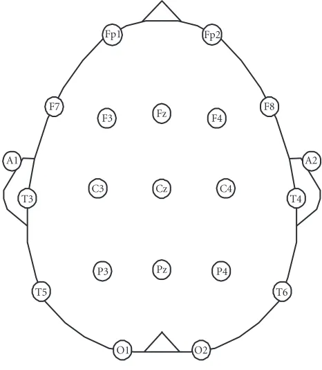
EEG signals are measured at the scalp by affixing an array of electrodes according to the 10-20 international system (Figure 1) and with reference to digitally linked ears (DLE).
DLE voltages are obtained by using the average of volt-ages at both earlobes as reference. The earlobes are selected because they constitute an almost quiet reference. In fact, they present small influences due to temporal activity [7].
If we denote byVe the voltage at any of the electrodes,
andVA1 andVA2 the voltages at the left earlobe and right earlobe, respectively, then the DLE-referenced voltage of
A1
Figure1: International 10-20 system of electrodes placement.
electrodeeis
whenVA1is the physical reference and
VDLE
whenVA2is the physical reference.
An EEG signal is thus composed of the DLE signals of each electrode. When a measure is composed of such single composite measures, it is called multivariate [8].
2.2. Training phase
The objective of this phase is two-fold: to extract EEG pat-terns that uniquely characterize MAs, and to train the sub-ject. The results of this phase are MA models that will serve as references for the application phase.
This phase can be performed with two approaches, namely, training without feedback and training with feed-back.
In the case of training without feedback, the subject is asked to perform MAs during a given period of time (with repetitions if necessary) while his EEG signals are recorded for ulterior MA model construction.
tk tk+1
Time
Sk EEG signals
T T1
Sk+1
Sk
Xk
Fk
Preprocessing
Pattern estimation
Pattern classification MA models
Computer action (k)
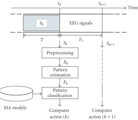
Computer action (k+ 1) Figure2: Basic scheme of a BCI in its application phase.
was successfully identified (positive feedback) or not (neg-ative feedback). According to neuroscience results [9,10], the human brain is able to modulate its activity in order to minimize the number of negative feedbacks. Training with feedback is possible only if an MA model exists, that is, the information of a previous training without feedback is available.
2.3. Application phase
The basic scheme of a BCI in its application phase is shown in Figure 2. The computer action at recognition timetkis
gen-erated by the classification of the EEG pattern present in the EEG signals (Sk) recorded during the T seconds preceding
the recognition time. In the sequel, we will call this EEG seg-ment of durationTa trial.
The time interval between two successive recognition times is denoted byTI (interaction period or computer
ac-tions period). The choice ofTIandTis the result of a
trade-offbetween computer actions rate, EEG pattern misclassifi-cation probability, and computational cost.
As EEG signals are contaminated by noise, a preprocess-ing step is necessary. The trial Skis then passed trough the
preprocessing module whose output is a clean trialXkor a
special message ifSkis too perturbed to be useful.
The pattern estimation module extracts the EEG patterns
Fk contained inXk. The nature ofFk is determined by the
classification algorithm.
Finally, a classifier module decides which computer ac-tion to consider based on a distance measure between MA model representatives and the patternFk.
3. PROPOSED BCI SYSTEM
3.1. BCI-system modules
According toFigure 2, a BCI in its application phase is com-posed of the following modules:signal acquisition,
preprocess-ing, pattern estimation, pattern classification, and computer actions generator.
In the training phase, the same modules are used plus an MA model builder. The role of the computer actions genera-tor is however different here as it is used to display visual cues (indicating which MA to perform) and to provide feedback.
Since BCI technology is still in its experimental phase, these modules and their relationships should be as flexible as possible.
3.2. OMs of the BCI
Five OMs1were implemented; they allow the subjects to
per-form various experiments from simple to more complex.
Visualization OM (VOM)
In this OM, the subject can watch a visual representation of his EEG in real time. Specific EEG features, such as the power values in the typical frequency bands (δ, θ, α, β), interelec-trode coherences, and total power at a given elecinterelec-trode, are mapped to a 3D virtual environment and are regularly up-dated. The objectives of this OM are to familiarize the subject with the system as well as to calibrate the latter.
Training without feedback OM (NFOM)
In this OM, the subject is asked (by means of visual or audio cues) to perform a defined MA. The produced EEG is then recorded for offline MA model construction.
Training with feedback OM (FOM)
The subject is asked to perform an MA and a feedback is pro-vided. This feedback is positive when the computer recog-nizes the MA and is negative otherwise. This is possible as MA models were calculated during a previous training with-out feedback. MA models can be updated in the course of a FOM (dynamic update) or at the end of it [11].
Control OM (COM)
Since the results of previous OMs are MA models, the sub-ject can start to control the system by performing the MAs for which the system has been trained. In this OM, visual or sound cues are no longer necessary.
Multisubject simultaneous training OM (MUOM)
This is a particular form of the FOM. It consists in a multi-subject game whose goal is to gain control of an object by performing an MA. This OM was chosen because of its more stimulating effect when compared to a simple feedback.
3.3. System architecture
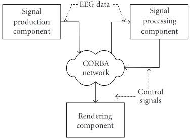
We grouped the system modules listed before into three com-ponents: signal production, signal processing, and multime-dia renderer.
EEG data Signal
production component
Signal processing component
CORBA network
Control signals Rendering
component
Figure3: BCI-system architecture.
We propose a distributed architecture in which each component offers specific services to the others in an efficient and transparent way.
Figure 3depicts the architecture diagram of our BCI sys-tem.
(1) The signal production component is responsible for signal acquisition, digitalization, and efficient data transmis-sion through the network.
(2)The signal processing componentis in charge of signal preprocessing, pattern extraction, MA model construction, and pattern classification.
(3)The rendering componentis used to display multime-dia cues in NFOM and FOM, as well as to provide the feed-back for the FOM. Furthermore, it acts as renderer in the VOM, COM, and MUOM.
The communication rules between these components were designed over the CORBA specification [12], and im-plemented in JAVA (for networking) and C and Matlab (for processing).
4. EEG SIGNALS PREPROCESSING
The purpose of EEG signal preprocessing is to maximize the signal-to-noise ratio (SNR). Noise sources can be nonneural (eye movements, muscular activity, 50 Hz power-line noise) or neural (EEG features other than those used for control) [6].
In this research, we centered our analysis on nonneu-ral noise such as eye-movement artefacts, muscular artefacts, and the 50 Hz power-line noise.
Since the frequencies of interest in EEG are mainly lo-cated below 40 Hz, we filtered the signals between 1 and 40 Hz. The 50 Hz power-line noise was therefore attenuated. For eye-movement artefacts and muscular artefacts, we chose to reject a trial containing any of these artefacts and, consequently, such a trial could not generate any computer action.
In the case of muscular activity, one of the best ap-proaches for detection consists in using independent com-ponent analysis (ICA) of EEG. However, ICA is basically an offline method since it is only meaningful when the amount of data is large enough [13].
0 1 2 3
0.5 s Fp1
Fp2
EEG trial contaminated by an eye blink
Figure4: Rejection of an EEG trial contaminated by an eye-blink artefact.
A practical method for detecting muscular artefacts is based on the fact that these artefacts are characterized by high frequencies (above 20 Hz) and high amplitudes. In [14], muscle artefact detection is achieved by considering the ab-solute and relative power over 25 Hz. In this paper, we set a threshold on the power at this frequency band based on vi-sual inspection and ICA during a calibration step.
For eye-movement artefacts detection, many methods have been proposed [15]. They are fundamentally offline be-cause they are mainly oriented to clinical research.
We implemented a method based on the power at pre-frontal electrodes (Fp1 and Fp2) because eye-movement artefacts are characterized by an abrupt change in amplitude mainly localized at Fp1 and Fp2 (Figure 4). The signal power at Fp1 and Fp2 is computed every half second and compared to the mean power of the preceding two seconds. If the cur-rent power subtracted from the mean is larger than some multiple of the standard deviation of the two-second power, the trial is marked as contaminated by an eye artefact and thus rejected. The threshold is determined in the calibration step.
5. EEG SIGNALS CLASSIFICATION
The classification of EEG signals based on the patterns char-acterizing the MAs constitutes a fundamental part of a BCI. As a matter of fact, the choice of the temporal parametersT
andTIis strongly dependent on the classification method.
An EEG signal is multivariate because it is composed of signals coming from several electrodes. In this paper, we pro-pose a decomposition of the multivariate classification into univariate classifications.Figure 5depicts the general scheme of our method.
Multivariate signals
Figure5: The MVSs classification problem is transformed into sev-eral univariate signal classifications.
5.1. Univariate signal classification in the time-frequency domain
In this subsection, the objects to be classified are univariate-signals (henceforth simply called univariate-signals).
Time-frequency representation
Time-frequency representations (TFRs) of a signal can be divided into two groups according to the nature of their transformations: linear (short-time Fourier transform), and quadratic (based on the Wigner-Ville distribution). Here we focus on the quadratic representation.
According to [16], all TFR of a signals(t) can be obtained ally called doppler),θis the frequency lag (usually called de-lay), andφ(θ, τ) is a two-dimensional function called the ker-nel.
The choice of the kernel is guided by the desire to have a TFR satisfying some established properties with regard to the application. Here, we designed a kernel with the objective of efficient signal classification.
There are a number of alternative ways for writing the general class of time-frequency distributions that are the most convenient for the classification application. One of them is the characteristic function (CF) formulation. We re-call that the CFM(θ, τ) is the double Fourier transform of
2All the integrals where the limits are not indicated span from−∞to +∞.
Combining (3) and (4), we obtain
M(θ, τ)=φ(θ, τ)
whereA(θ, τ) is the symmetrical ambiguity function (AF) of
s(t), defined as
Equation (6) allows us to interpret the AF as a measure of the joint time-frequency auto-correlation ofs(t). Theθ−τ
plane is commonly called ambiguity plane.
The kernel function that can be seen as a mask in the ambiguity plane has the goal of enhancing the regions in the planeθ−τthat better discriminate the signals to be classified. In this research, we consider the classification problem with respect to the modulus of the CF. The kernel is then designed so as to enhance the regions where this modulus is more discriminative.
Kernel design Given a training set
Υ=sq1
of labeled signals, whereWis the number of classes,Qwkthe number of labeled signals belonging to classwk, andsqwkk(t) theqkth signal belonging to classwk, we wish to determine a
kernel functionφ(θ, τ) so that we can compare the CF mod-ulus of an unknown signals(t) to that of each class and assign
s(t) to its most likely class.
In order to detect the regions where the class differences are maximal, we define the contrast functionΓ(θ, τ) as
where
is the mean AF modulus corresponding to classwk. The
vari-ance of the AF modulus corresponding to classwkis
VARAwk(θ, τ)
The discrete version of theθ−τplane allows us to select theκpoints of maximum contrast.
We group these points in a max-contrast setKdefined as
K=m1·∆θ, n1·∆τ
where∆θand∆τare the discretization steps.
We design the kernel as a discrete binary function, where the points inKare set to “1” while the others are set to “0,”
0 otherwise. (15)
Class model
The model of the classwkis composed of its mean AF
mod-ulus, its variance AF modmod-ulus, and the kernel. All these ele-ments are considered in their discrete form.
By an adequate choice of units, we can set the discretiza-tion steps∆θand∆τto 1.
The model of the classwkcan be written as follows:
Modelwk
=EAwk(m, n),VARAwk(m, n),
φ(m, n). (16)
In an alternative way, the setKcan be included instead of
φ(m, n) as follows: a distance measure betweens(t) and a class model. We take
as a distance measure
ds(t),modelwk
wk is the Mahalanobis distance between the AF modulus ofs(t) and the mean AF modulus of classwkat the
points where the kernelφ(m, n) is different from zero. The most likely class ofs(t) is given by its classification defined by
The classification error rate is defined, with respect to a la-beled signal set (test set), by the ratio between the number of correctly classified signals and the total number of signals in the labeled set.
The choice of the parameterκ(number of contrast points that we take into account) remains to be detailed. This pa-rameter should be chosen so as to minimize the classification error in a test set of labeled signals. This can be achieved by increasing the value ofκuntil a minimal classification error rate is obtained.
5.2. MVS classification in the time-frequency domain A MVS S(t) can be written in a vector form S(t) =
[s1(t), . . . , sN(t)]t, where the si(t) are the components of
S(t). We can easily adapt the formulation of the univariate-classification problem inSection 3.1to the multivariate case as follows.
Given a training set of labeled MVSs
Υ=Sq1
where W is the number of classes, Qwk the number of la-beled MVSs belonging to classwk, andSqwkk(t) theqkth MVS
belonging to class wk, we wish to characterize each class
by a model so that we can compare an unknown MVSS(t) to each class-model and assign S(t) to its most likely class.
Time-frequency-space representation of MVS
The multivariate ambiguity function (MAF) of an MVSS(t) is defined by [17]
MA(θ, τ)=
Another way to write (21) in a matrix form is presented
In (22), the terms on the diagonal are the auto-ambiguity functions (commonly called AFs) and the off-diagonal terms are called cross-ambiguity functions.
InSection 5.1we mentioned the fact that the AF could be interpreted as a measure of the joint time-frequency auto-correlation. The generalization of this interpretation implies that the MAF is an indicator of the joint time-frequency-space autocorrelation of a MVS. The time-frequency-space dimension is taken into account by the cross-ambiguity functions.
Spatial decorrelation
A common approach when dealing with multivariate data is to find a number of components satisfying some statistical properties that can generate the original multivariate data by applying a linear transformation. The most common tech-niques are the principal component analysis (PCA) whose components are linearly statistically independent and ICA whose components are statistically independent.
In both PCA and ICA the correlation between the new transformed components (TRCs) is zero. Therefore, PCA and ICA lead to MVSs whose components are spatially decor-related.
Furthermore, the MAF matrix of a spatial decorrelated MVS is diagonal.
Besides PCA and ICA, other decorrelation methods can be used. As in the case of the kernel design, we can design a decorrelation method whose goal is to find components that maximally discriminate among the classes. A way to achieve this goal is to use a feature extraction based on eigenvector analysis [18]. An example of application in the BCI frame-work can be found in [19], where an interpretation in terms of spatial filters is presented. However, only two classes can be classified at a time.
We present below a decorrelation method based on the joint diagonalization of the autocorrelation matrices of each class.
We denote byZ(t) the transformed MVS (TMVS) result-ing from the premultiplication ofS(t) by the matrixP:
Z(t)=P·S(t). (23)
The labeled MVS belonging to the training setΥareP -projected to generate the following transformed setPΥ:
PΥ=Zq1
The signal components (transformed components) of
Zqk
wk(t) are{z
qk
wk(t); 1≤≤N}.
The discrete version of the setPΥis constituted of the matricesZqk
wkwhose elements are the values ofZ
qk
wk(t) at the sampling instants.
We wish to determine the matrixPsuch that
EZwk·Zwtk
where Dwk are diagonal matrices and Rwk are called the autocorrelation matrices of the classwk. Thus the matrixP
simultaneously diagonalizes the set{Rwk|1≤k≤W}. As a matter of fact, the matrix P that exactly diago-nalizes this set exists when the Rwk are normal
3
commut-ing matrices [20]. Accordcommut-ing to (25), the Rwk are normal but they do not necessarily commute. However, it is pos-sible to find a matrix that approximately diagonalizes the set {Rwk | 1 ≤ k ≤ W} [20] by optimizing a joint di-agonality criterion (minimization of the square sum of the off-diagonal elements). An iterative procedure consisting in the application of plane rotations so as to satisfy the joint-diagonality criterion is presented in [20]. Because of the effi -ciency and the good results of such method, we used it in our work.
In order to characterize the discrimination potential of each of the components ofZ(t), we define the contrast func-tionΩ(), where =1, . . . , N is the TRC index, as follows:
The functionΩ() measures the contrast of theth trans-formed component when the energy in that component is used as a discrimination parameter between the classes.
The contrast measure allows us to assign to each trans-formed component (27) a classification weight
ρ= Ω
The model of the classwkis composed of the projection
ma-trixP, the set of classification weights{ρ |1≤≤N}, and
the univariate model of each component (seeSection 5.1): spectively, the mean AF modulus of theth component as-sociated to the classwk, the variance AF modulus of theth
associated to the classwk, and the max-contrast set of theth
component.
Unlabeled signals classification
Given an MVSS(t), we first compute its TMVS Z(t) (see (23)) and obtain the TRCs z1(t), z2(t), . . . , zN(t). Then the
distances between each component and the model of each class associated with that component are calculated as fol-lows:
The most likely class ofS(t) is given by its classification defined as
6. EXPERIMENTAL METHODS AND PROTOCOL
Two male and healthy volunteers (S1 and S2), 29 and 23 years old, participated in six sessions of 20 minutes distributed over five weeks. The subjects were comfortably sitting in an armchair and placed in front of a computer screen. The ex-perimentation room was quiet and slightly illuminated.
The subjects started each session by five minutes of the VOM. During the VOM, we controlled the recording condi-tions and set the threshold parameters for artefact rejection (see Section 4). Furthermore, the VOM allowed subjects to get familiar with the system.
The EEG signals were recorded with reference to DLE (seeSection 2.1) and from electrodes Fp1, Fp2, F3, F4 C3, C4, P3, P4, O1, and O2 of the 10/20 international system, at a rate of 256 Hz per channel. The electrodes Fp1 and Fp2 were used only for eye-movement artefacts detection and they were not included in the classification analysis.
Both subjects were asked to perform the following imag-ined MAs: vertical movements of the left and right index fingers (MA1 and MA2) and incremental mental counting (MA3).
Visual cues were used to indicate which MA to perform. In the case of MA1 and MA2, a horizontal arrow pointing to the left or to the right was displayed on the computer screen; for MA3, the first two-digit number was displayed.
The first recording session was carried out without feedback and the next five with feedback. In the first ses-sion, the first MA models were calculated; this allowed us to provide feedback in the second session. During the feedback sessions, the MA models were updated incrementally as ex-plained inSection 6.2.
The temporal parametersTandTI were both set to 0.5
second (seeSection 2.3). The goal was therefore to train MA models able to correctly classify half-second EEG segments (trials).
6.1. Protocol of a training-without-feedback session
The first five minutes were spent with the VOM. The remain-ing 15 minutes were divided into three five-minute slices in which, respectively, MA1, MA2, and MA3 were trained.
The five-minute slices were as well divided into one-minute recordings and thirty-second break as depicted in Figure 6. The one-minute recordings were organized in the following way. At the beginning, the corresponding visual cue was displayed and lasted five seconds. Then a break sig-nal appeared, indicating five-second break. This process was repeated during the one-minute recording (Figure 6).
At the end of this session, the MA models for the three MAs were computed. These models are calculated as ex-plained inSection 5.
Theoretically, we have 180 trials per MA for training the MA models. However, the first trial after the presentation of the visual cue is rejected because of the presence of evoked potentials—due to visual stimulation—and about 20% of the trials are rejected because of artefacts. In practice, no more than 150 trials per MA were available.
6.2. Protocol of a training-with-feedback session
The twenty minutes are distributed between visualization, MAs, and breaks in the same way as in the precedent case (Figure 7).
During the MAs, a feedback is provided to the subject in the form of a sphere that moves left, right, or upwards if MA1, MA2, or MA3 are correctly identified. If the MA is wrongly classified, the sphere does not move. The feedback is provided for each half second but the first after the visual cue indicates which MA to perform (seeFigure 7).
During the last break period of each five-minute slice, the MA models are updated with the new recorded data.
Table 1 shows the MAs that were trained in each five-minute slices of the session with feedback.
7. RESULTS AND DISCUSSIONS
Recording session
Visualization modality 5-minute slice 5-minute slice 5-minute slice
0 5 10 15 20
minutes
Five-minute slice 1-minute recording Break
1-minute recording Break
1-minute
recording Break
0 1.0 1.5 2.5 3.0 4.0 5.0minutes
One-minute recording
Visual cue Mental
activity Break
Mental activity Break
0 5 10 50 55 60seconds
Break cue
Figure6: Training-without-feedback protocol.
Recording session
Visualization modality 5-minute slice 5-minute slice 5-minute slice
0 5 10 15 20minutes
Five-minute slice 1-minute recording Break
1-minute recording Break
1-minute
recording Break
0 1.0 1.5 2.5 3.0 4.0 5.0minutes
One-minute recording
Visual cue Mental
activity Break
Mental activity Break
0 5 10 50 55 60seconds
Break cue MA with feedback
0 0.5 1.0 1.5 2.0 2.5 3.0 3.5 4.0 4.5 5.0seconds Visual cue
TRC 8 TRC 7 TRC 6 TRC 5 TRC 4 TRC 3 TRC 2 TRC 1
S1
Transformed components classification weights
0.13
0.03 0.04
0.24
0.03
0.21
0.20
0.14
F3 F4 C3 C4 P3 P4 O1 O2
Figure8: Results for S1. Left: structure of the matrixP. Right: classification weights of each TRC.
TRC 8 TRC 7 TRC 6 TRC 5 TRC 4 TRC 3 TRC 2 TRC 1
S2
Transformed components classification weights
0.14
0.05
0.20
0.04
0.06
0.21
0.19
0.10
F3 F4 C3 C4 P3 P4 O1 O2
Figure9: Results for S2. Left: structure of the matrixP. Right: classification weights of each TRC.
First session (without feedback)
The number of retained trials in the first session (after arte-fact rejection) per subject and per MA is reported inTable 2. We used 100 trials to compute the matrixP, the mean
Table1: MAs trained during the three five-minute slices of each feedback session.
Session
2 3 4 5 6
5-min
slic
e 1 MA1 MA2 MA3 MA1 MA2
2 MA2 MA2 MA3 MA1 MA1
3 MA3 MA3 MA1 MA2 MA3
Table2: Number of retained trials per subject and per MA in the first session (after artefact rejection).
Mental activity
MA1 MA2 MA3
Su
b
je
ct S1 149 144 148
S2 146 143 142
In Figures8and9(for S1 and S2, respectively), the ab-solute values of the coefficients of the matrix P are repre-sented in a comparative graph (left). This graph gives us the information about the composition of each TRC as a linear combination of signals coming from different electrodes. In the right part, the classification weights associated with each TRC, calculated according to (27), are depicted.
The results of Figures8and9show that for both subjects there are five TRCs that seem to be more important for the classification than the others (1, 2, 3, 5, and 8 for S1, and 1, 2, 3, 6, and 8 for S2). In order to confirm this impression, we computed the classification error associated with each TRC and the optimal number of contrast points. These results are shown in Figures 10 and11 (for S1 and S2, respectively). From these results, we can say that the smaller error rates correspond to those components with largest classification weights.
We also present the optimal contrast points for the four TRCs that have the smallest error rate. Only the first quad-rants were represented since the modulus of the AF is sym-metric with respect to the origin.
Sessions from two to six (with feedback)
InTable 3, we report the number of retained trials after arte-fact elimination for each five-minute slice from sessions two to six.
During the second session, each MA was trained with feedback (seeTable 1). Such feedback was produced by tak-ing as reference the models built after the first session. In Table 4, we present the percentage of trials that were not correctly classified among the nonrejected trials (error rate).
Table3: Number of retained trials after artefact elimination in the sessions where feedback was provided.
S1
Session
2 3 4 5 6
5-min
slic
e 1 145 141 142 147 148
2 147 151 144 148 144
3 150 152 150 149 146
S2
Session
2 3 4 5 6
5-min
slic
e 1 146 144 146 144 149
2 142 145 148 148 139
3 145 147 143 142 150
Table4: Percentage of misclassified trials during the second session (first session where feedback was provided). The MA models used for producing feedback were built after the first session where no feedback was provided.
Subject
1 2
5-min
slic
e 1 28 36
2 26 34
3 23 28
At the end of the second session, new MA models were built using 100 trials (randomly chosen) to compute the matrix P, the mean AF modulus, and the variance AF modulus. The test set composed of the remaining tri-als was used to compute the optimal number of contrast points.
S1
0 31.2 62.5 125 156.2 218.7 250 ms 16
32 48 64 80 96 112 128 Hz
TC1 (188 points)
0 31.2 62.5 125 156.2 218.7 250 ms 16
32 48 64 80 96 112 128 Hz
TC2 (156 points)
0 31.2 62.5 125 156.2 218.7 250 ms 16
32 48 64 80 96 112 128 Hz
TC3 (172 points)
0 31.2 62.5 125 156.2 218.7 250 ms 16
32 48 64 80 96 112 128 Hz
TC5 (200 points)
1 2 3 4 5 6 7 8
20 22 19
31
14
36
32
30 Transformed components error rates
Figure10: Top: contrast points selected for the four TRCs with the smallest error rates (as the modulus of the AF is symmetric with respect to the origin, only the first quadrant is represented). Down: error rates associated with each TRC (S1).
It is important to note that we built new MA models at the end of the second session in order to make it in feed-back conditions. In this way, it is possible to update the models after each five-minute slice in sessions from three to six.
In sessions from three to six, we updated the matrixP, the mean AF modulus, and the variance of the AF modu-lus of the trained MA for each five-minute slice. This pro-cedure was performed by using 100 trials randomly chosen to update those parameters and to take the remaining trials as a test set for determining the optimal number of contrast points.
In Figures14and15(for S1 and S2, respectively), we rep-resent the evolution of the error rate over the sessions from three to six. These results for each five-minute slice are re-ported inTable 1.
As it can be seen, the error rate decreased almost al-ways except between sessions 3 and 4 for S1. Neverthe-less, at the end of the sixth session, we achieved the low-est error rates for all the MAs. This result sugglow-ests that the feedback strategy improved the performance of the sys-tem. In fact, the subjects reported their general satisfac-tion with regard to feedback because of its stimulating ef-fects.
8. CONCLUSIONS AND FUTURE WORK
S2
0 31.2 62.5 125 156.2 218.7 250 ms 16
32 48 64 80 96 112 128 Hz
TRC 3 (180 points)
0 31.2 62.5 125 156.2 218.7 250 ms 16
32 48 64 80 96 112 128 Hz
TRC 6 (152 points)
0 31.2 62.5 125 156.2 218.7 250 ms 16
32 48 64 80 96 112 128 Hz
TRC 2 (260 points)
0 31.2 62.5 125 156.2 218.7 250 ms 16
32 48 64 80 96 112 128 Hz
TRC 8 (172 points)
0 31.2 62.5 125 156.2 218.7 250 ms 16
32 48 64 80 96 112 128 Hz
TRC 1 (200 points)
Doppler Delay
1 2 3 4 5 6 7 8
28
25
21
31 30
22
38
30 Transformed components error rates
Figure11: Top: contrast points selected for the four TRCs with the smallest error rates (as the modulus of the AF is symmetric with respect to the origin, only the first quadrant is represented). Down: error rates associated with each TRC (S2).
In order to familiarize the subjects with our BCI, we pro-posed to precede each session with a short real-time visual-ization of a projection of the EEG signals in a 3D environ-ment.
We classified EEG signals from the point of view of the joint correlation in three dimensions: time, frequency, and space (as EEG signals are multivariate). In order to reduce the amount of data that results from such analysis, we decor-related the EEG signals before moving to the time-frequency correlation part. The decorrelation process resulted in a set of TRCs. In this way, we divided the original problem of clas-sification of MVSs into several univariate clasclas-sifications.
The training was performed in two ways: with and
with-out feedback. The obtained results show that the relation-ship between the TRCs remains essentially the same for both training types.
Nevertheless, as noticed in [11] the structure of the MA models is different from person to person. Therefore, a BCI should be personalized.
The general reduction of the classification error rate over the sessions where feedback was provided shows that the feedback constituted an effective strategy for the training. Nevertheless, more experiments are necessary for confirm-ing this hypothesis.
S1
0 31.2 62.5 125 156.2 218.7 250 ms 16
32 48 64 80 96 112 128 Hz
TRC 5 (212)
0 31.2 62.5 125 156.2 218.7 250 ms 16
32 48 64 80 96 112 128 Hz
TRC 3 (164)
0 31.2 62.5 125 156.2 218.7 250 ms 16
32 48 64 80 96 112 128 Hz
TRC 2 (160)
0 31.2 62.5 125 156.2 218.7 250 ms 16
32 48 64 80 96 112 128 Hz
TRC 1 (176)
0 31.2 62.5 125 156.2 218.7 250 ms 16
32 48 64 80 96 112 128 Hz
TRC 8 (196)
Doppler Delay
F3 F4 C3 C4 P3 P4 O1 O2
TRC 5
TRC 3
TRC 2
TRC 1
TRC 0
0.34
0.27
0.14
0.12
0.10
Transformed components classification weights
Figure 12: Results for S1. TRCs with largest classification weights for the MA models built after the second session (first session with feedback). Top: contrast points in the Doppler-delay plane. Middle: rows of the matrixPassociated with the TRCs. Down: classification error rate associated with each TRC.
As the goal is to control devices by thinking, it is necessary to add more MAs for making, at least, a two-dimensional control possible.
We will consider other spatial analysis techniques such as nonlinear PCA for extracting those TRCs that can be
classi-fied in the time-frequency domain.
S2
0 31.2 62.5 125 156.2 218.7 250 ms 16
32 48 64 80 96 112 128 Hz
TRC 3 (184)
0 31.2 62.5 125 156.2 218.7 250 ms 16
32 48 64 80 96 112 128 Hz
TRC 6 (224)
0 31.2 62.5 125 156.2 218.7 250 ms 16
32 48 64 80 96 112 128 Hz
TRC 2 (152)
0 31.2 62.5 125 156.2 218.7 250 ms 16
32 48 64 80 96 112 128 Hz
TRC 8 (208)
0 31.2 62.5 125 156.2 218.7 250 ms 16
32 48 64 80 96 112 128 Hz
TRC 1 (232)
Doppler Delay
F3 F4 C3 C4 P3 P4 O1 O2
3
6
2
8
1
0.22
0.21
0.17
0.16
0.16 Transformed components
classification weights
Session 3 Session 4 Session 5 Session 6 MA 3
MA 2
MA 1
S1
22 24 20 20
26 22
19 15
25 24 21 17
Figure 14: Error rate evolution for S1 over the training sessions from three to six. We reported the error rate for each five-minute slice inTable 1.
Session 3 Session 4 Session 5 Session 6 MA 3
MA 2
MA 1
S2 25 23 21
20
34
28 25 25
30 28 25
23
Figure 15: Error rate evolution for S2 over the training sessions from three to six. We reported the error rate for each five-minute slice inTable 1.
ACKNOWLEDGMENTS
We wish to acknowledge Patrick Aebischer and Guy Courbe-baisse for fruitful discussions and suggestions which allowed us to improve the performance of our system. We would also like to thank the persons that participated in the experimen-tal sessions.
REFERENCES
[1] J. D. Bayliss,A Flexible Brain-Computer Interface, Ph.D. thesis, University of Rochester, Rochester, NY, USA, 2001.
[2] M. Middendorf, G. McMillan, G. Calhoun, and K. S. Jones, “Brain-computer interfaces based on the steady-state visual-evoked response,” IEEE Transactions on Rehabilitation Engi-neering, vol. 8, no. 2, pp. 211–214, 2000.
[3] A. K¨ubler, B. Kotchoubey, H.-P. Salzmann, et al., “Self-regulation of slow cortical potentials in completely paralyzed human patients,”Neuroscience letters, vol. 252, no. 3, pp. 171– 174, 1998.
[4] G. Pfurtscheller, C. Neuper, C. Guger, et al., “Current trends in Graz brain-computer interface (BCI) research,” IEEE Transactions on Rehabilitation Engineering, vol. 8, no. 2, pp. 216–219, 2000.
[5] D. J. McFarland, G. W. Neat, R. F. Read, and J. R. Wolpaw, “An EEG-based method for graded cursor control,”Psychobiology, vol. 21, no. 1, pp. 77–81, 1993.
[6] J. R. Wolpaw, N. Birbaumer, W. J. Heetderks, et al., “Brain-computer interface technology: a review of the first interna-tional meeting,”IEEE Transactions on Rehabilitation Engineer-ing, vol. 8, no. 2, pp. 164–173, 2000.
[7] D. J. McFarland, L. M. McCane, S. V. David, and J. R. Wolpaw, “Spatial filter selection for EEG-based communication,” Elec-troencephalography and Clinical Neurophysiology, vol. 103, no. 5, pp. 386–394, 1997.
[8] J. F. Hair Jr., R. E. Anderson, R. L. Tatham, and W. C. Black, Multivariate Data Analysis, Prentice Hall, Upper Saddle River, NJ, USA, 1998.
[9] J. R. Evans and A. Arbarbanel, Eds., Introduction to Quan-titative EEG and Neurofeedback, Academic Press, San Diego, Calif, USA, 1999.
[10] J. Robbins,A Symphony in the Brain, Atlantic Monthly Press, New York, NY, USA, 2000.
[11] G. Garcia, T. Ebrahimi, and J.-M. Vesin, “Classification of EEG signals in the ambiguity domain for brain com-puter interface applications,” inProc. 14th International Con-ference in Digital Signal Processing, Santorini, Greece, July 2002.
[12] M. Henning and S. Vinoski, Advanced CORBA Program-ming with C++, Addison-Wesley professional computing se-ries. Addison-Wesley, Boston, Mass, USA, 1999.
[13] T.-P. Jung, C. Humphries, T.-W. Lee, et al., “Extended ICA removes artifacts from electroencephalographic recordings,” inAdvances in Neural Information Processing Systems, vol. 10, pp. 894–900, MIT Press, Cambridge, Mass, USA, 1998. [14] M. van de Velde, G. van Erp, and P. J. Cluitmans, “Detection
of muscle artefact in the normal human awake EEG,” Elec-troencephalography and Clinical Neurophysiology, vol. 107, no. 2, pp. 149–158, 1998.
[15] L. Vigon, R. Saatchi, J. E. W. Mayhew, and R. Fernandes, “A quantitative evaluation of techniques for ocular artefact filter-ing of EEG waveforms,” IEE Proc. Science Measurement and Technology, vol. 147, no. 5, pp. 219–228, 2000.
[16] L. Cohen,Time Frequency Analysis, Prentice Hall Signal Pro-cessing Series. Prentice Hall, Upper Saddle River, NJ, USA, 1995.
[17] M. G. Amin, A. Belouchrani, and Y. Zhang, “The spatial am-biguity function and its applications,” IEEE Signal Processing Letters, vol. 7, no. 6, pp. 138–140, 2000.
[18] C. W. Therrien, Decision Estimation and Classification, John Wiley & Sons, New York, NY, USA, 1989.
[19] H. Ramoser, J. M. Gerking, and G. Pfurtscheller, “Opti-mal spatial filtering of single trail EEG during imagined hand movement,”IEEE Transactions on Rehabilitation Engineering, vol. 8, no. 4, pp. 441–446, 2000.
Gary N. Garcia Molinawas born in Sucre, Bolivia. He received his M.S. degree in elec-trical engineering from the Swiss Federal Institute of Technology, Lausanne (EPFL), in 2001. His diploma work was on the ap-plication of pattern recognition techniques to speech processing. He then worked as a Software Engineer in the design and imple-mentation of distributed systems for mul-timedia content broadcasting. Since April
2001, he has been a Ph.D. student at EPFL where he is involved in several projects in image, video, and biomedical signal processing. Currently he develops an adaptive direct brain-computer commu-nication device with strong emphasis on the models and interpre-tations of synchronized neural activity.
Touradj Ebrahimi received his M.S. and Ph.D. degrees, both in electrical engineer-ing, from the Swiss Federal Institute of Technology, Lausanne (EPFL), in 1989 and 1992, respectively. In 1993, he was a Re-search Engineer at the Corporate ReRe-search Laboratories of Sony Corporation in Tokyo, where he conducted research on advanced video compression techniques for storage applications. In 1994, he was a Researcher
at AT&T Bell Laboratories working on very low bitrate video cod-ing. Ebrahimi is currently a Titular Professor at the School of En-gineering, Signal Processing Institute of EPFL, where he is involved in research and teaching of multimedia information processing and coding. In 2002, he founded Emitall, a research and development company in electronic media innovations. Ebrahimi was the recip-ient of the IEEE and Swiss national ASE award in 1989, and the winner of the first price for the best paper appeared in IEEE Trans-actions on Consumer Electronics in 2001. In 2001 and 2002, he received two ISO awards for contributions to MPEG-4 and JPEG 2000 standards. He is the author or coauthor of over 100 scientific publications and holds a dozen patents.
Jean-Marc Vesingraduated from the ´Ecole Nationale Sup´erieure d’Ing´enieurs Elec-triciens de Grenoble (ENSIEG, Grenoble, France) in 1980. He received his M.S. degree from Laval University, Qu´ebec city, Canada, in 1984, where he spent four years on re-search projects. After two years in indus-try, he joined the Signal Processing Insti-tute (ITS) of the Swiss Federal InstiInsti-tute of Technology, Lausanne, Switzerland, where