Modeling of The Fluid Solid Interaction during Seismic Event

20th International Conference on Structural Mechanics in Reactor Technology (SMiRT 20) Espoo, Finland, August 9-14, 2009 SMiRT 20-Division III, Paper 2661

Modeling of The Fluid Solid Interaction during Seismic Event

Jan Vachulka

Stevenson and Associates, Vejprnicka 56,Pilsen, Czech Republic, e-mail: [email protected]

Keywords: interaction, fluid, potential, finite element, boundary element.

1

ABSTRACT

The fluid solid interaction belongs to one of the important topics in structural design in nuclear field.

The main aim of this paper is to present acceptable method for determining fluid-structure interaction during seismic event using standard finite element code without implemented fluid finite elements. The method is based on assumption that in-vacuum modal shapes of the structure are known and also the modal shapes of the free liquid surface are known. The mode shapes in vacuum are determined by standard finite element code and free surface modes are derived analytically or using boundary element method. The boundary condition on the fluid-structure interface is obtained semi-analytically in form of Fourier or Bessel-Fourier series for simple domains or using boundary element method for complicated fluid domains. The fluid is assumed to be irrotational and incompressible. Applying Galerkin method the system of is obtained. The system of equations is solved in time domain using Newmark integration scheme.

The seismic response of the liquid-filled tank is calculated. The calculated example shows very good agreement with the previously published. The method can be used in nuclear technology design.

2

INTRODUCTION

The incompressible fluid solid interaction problems can be described using following sets of equations:

1) La-Place equation in fluid domain

"

!

=

0

2) Free surface condition of the fluid 0 2 2

=

! !

+

! !

t z

g " "

3) Fluid-solid interface equations

grad

( )

"

!

n

r

=

u

&r

!

n

r

4) Solid domain equations (Elasticity equations)

where

!

is fluid potential, ur is solid body displacement, nr is outer normal of fluid-solid interface

The sets of these equations can be solved using FEM, combination of the FEM and BEM or semianalitical methods in form of infinite series for simple domains can be used. Hence the majority of authors are focused on modal analysis of the fluid-solid systems Amabili (1996), Amabili (1998).

3

DESCRIPTION OF PROPOSED METHOD

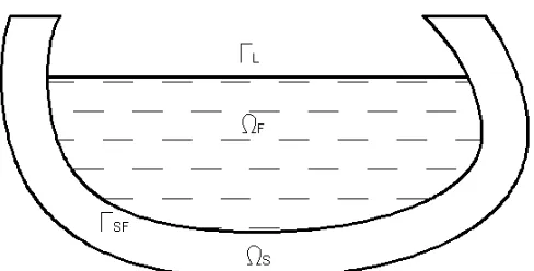
Figure 1. Fluid and solid domain

Summing up the above assumptions we have:

!

=

!

_S

+

!

_B

+

!

_R,

_"

_!

=

_"

(

_!

_S

+

_!

_B

+

_!

_R

)

=

0

(1)

Where

!

_S is convective part of fluid potential

"

!

_S

=

0

on

!

_F , (2)

0 n

S =

! !"

on

!

_SF. (3)

1) The impulsive part of the potential !_Bsatisfies (4), (5), (6):

0

B

=

!

"

on

!

F , (4)

( )

n

u

n

grad

n

B

B

r

&r

r

₌

_!

!

=

"

"

#

#

on

!

_SF, (5)

a

!

_B

=

0

on

!

_L. (6)

2) Rigidly impulsive part of the fluid potential

!

R satisfies (7), (8), (9):

0

R

=

!

"

on

!

F, (7)

( )

n

u

n

grad

n

R g

R

r

_&r

r

!

=

!

=

"

"

#

#

on

!

_SF (8)

0

R

=

!

on

!

L. (9)

3) All parts of potential are bound on the free surface

_!

_Lby following relationship (10)

0

g 1 n

) (

g 1

n S

R B S

= +

! + + ! = + ! !

"

"

"

"

"

"

&&

In equations (1)-(10)

u

&r

means the temporal derivative of the solid part displacement

g

u

&r

is the velocity of the seismic motion

nr is the outer normal of fluid-solid interface

S

!

,

!

F,

!

SF,

!

L are visible in Figure. 1

3.1 Numerical approach-weighted residual method

Applying weighted residuum approach, virtual works principle and relations (1)-(10) we get the equation for fluid domain (11) and solid domain (12).

0

d

g

1

d

n

d

n

d

n

L L L L L S S L S R L S B L S

S

+

=

!

!

+

!

!

+

!

!

"

"

"

"

# # # #

#

$%

%

#

$%

%

#

$%

%

#

$%

%

&

&

(11)

(

%

%

%

)

$

#

"

!

#

"

!

&

'

#

! $ !

d

)

u

u

(

u

d

n

u

d

S SF g s T S R B S T f s S T

(

(

(

r

*

r

=

)

r

r

&

+

&

+

&

)

r

&r

&

+

&r

&

(12)

Introducing the approximations of the solid and fluid region in form:

[ ] { }

N

r

(

t

)

r

u

r

=

r

_ST _U

!

(13)

[ ] { }

N

_S

s

(

t

)

S

=

!

"

(14)

[ ]

N

_B

{ }

r

(

t

)

B

=

!

&

"

(15)

g g

g u (t) r

ur = !r (16)

n

r

n

)

t

(

u

R _g

g R R

r

r

&

=

!

"

"

#

!

=

$

$

%

(17)

Substitution into equations (11) and (12) using Green theorem yields in (18)

[ ] [ ]

[ ] [ ]

{}

{}

[ ] [ ]

[ ] [ ]

{}

{}

[ ] [ ] [ ]

[ ]

[ ]

{}

{}

{ }

[ ]

{ }

[ ]

_!

"

#

$

%

&

'

(

)

*

+

,

-.

=

!

"

#

$

%

&

'

(

)

*

+

,

-

+

+

!

"

#

$

%

&

'

(

)

*

+

,

-+

!

"

#

$

%

&

'

(

)

*

+

,

-g g F A F T F

u

u

N

0

0

L

s

r

M

0

0

M

M

s

r

C

S

-S

C

s

r

K

0

0

K

&

&&

&&

&&

&

&

(18)

The particles of equation (18) are following:

[ ]

_!

[ ]

[ ]

" " # = L L S f T S f F d n N N K $

$

%

%

is stiffness matrix of the fluid (19)

[ ]

=

_!

[ ] [ ]

L L S T S f

F N N d

g M

"

"

#

{ }

_!

[ ]

" " #

= L

L R T S

f d

n N

N

$

$

%

&

is the load vector of the fluid (21)

[ ] [ ] [ ][ ]

=

_!

S

S T

d B D B K

"

"

is the stiffness matrix of the solid (22)

[ ]

=

_!

[ ]

"

{ } { }

" "

[ ]

SF

SF S T

s T U

f N r n N d

S

#

#

$

is the coupling matrix of the sloshing and bulging part of fluid

potential

[ ]

=

_!

[ ]

"

{ } { }

" "

[ ]

SF

SF B T

s T U f

A N r n N d

M

#

#

$

is added mass matrix (23)

[ ] [ ] [ ]

=

_!

S

S U s T

U N

N M

"

"

#

is the mass matrix of the solid (24)

{ }

=

_!

[ ]

"

{ } { }

" " " SF

SF R T

s T U f

1 N r n d

L

#

#

$

%

load vector of caused by fluid pressure (25)

{ }

=

_!

[ ]

{ }

{ }

S

S g T s T U s

2 N r r d

L

"

"

#

load vector of caused by solid inertia (26)

{ } { } { }

L

=

L

1

+

L

2 is the total load vector (27)

[ ]

C

is damping matrix of the solid

[ ]

C

F is damping matrix of the fluid

4

PRACTICAL USE OF THE PROPOSED METHOD

If we get input data in the form of the in vacuum modal shapes of the solid part and sloshing potential of the fluid in surrounded by a rigid solid, then applying the boundary conditions (5) and (6) the values of

!

B can

be obtained. Similarly the values of

!

_R can be get from boundary conditions (8) and (9). The input modal shapes can be the functions (especially polynomial) or the nodal displacements( if we use a FEM code). The fluid domain can be simple (rectangular, circular, spherical) and the values for

!

B and

!

R can be get in

closed form or for complicated domains using boundary integral techniques. The problems lead to system of linear equations if BEM is applied.

The values of

!

_S for rigid solid domains can be get in closed form for simple domains or using boundary integral techniques for complicated domains. The problem leads to eigen-value solution. This results from equations (2),(3) and (10) assuming no seismic motion and rigid walls of the solid part.

Having all the parts of fluid potential and in vacuum modal shapes the fluid-structural matrices can be assembled and seismic FSI problem can be solved.

5

THE RESULTS AND COMPARISONS

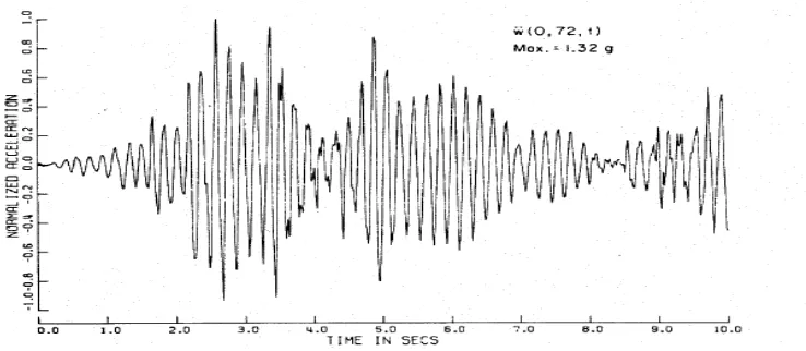
Example

Previously published seismic response of the tall radial storage tank with rigid bottom was chosen as an

example. The radial time histories of the top of the tank were compared. The tank was loaded only in

horizontal direction, input motion was EL-Centro. The diameter of tank was 14.604m, height 21.9456m, thickness of the shell 25.4mm. The tank was made of steel and full of the water. Relative damping ratio 2% was considered. First five members of Fourier-Bessel-series were chosen for approximation of the fluid

potentials. The effect of sloshing was not taken into account. The FEM model was constructed using the shell elements in order to calculate in vacuum modal shapes and can be seen on Fig. 2.

Figure 2. Finite element model of the storage tank

Figure 4. Time history of acceleration of the top of tall storage tank published by Haroun (1980)

ar

-15 -10 -5 0 5 10 15

0 1 2 3 4 5 6 7 8 9 10

ar

Figure 5. Time history of acceleration of the top of tall storage tank calculated using proposed method

rs! "0 ,rs! "1 ,rs! "2

(

)

rs! "0 ,rs! "1 ,rs! "2

(

)

rs! "0 ,rs! "1 ,rs! "2

(

)

Table 1. Table comparison of the response of the top of the tank

Response Proposed method Haroun (1980) Difference

Radial displacement (mm) 11 11.30 2.7%

Radial acceleration (ms-2) 13.19 12.95 1.8%

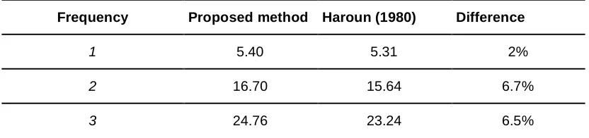
Table 2. Table comparison of fundamental frequencies

Frequency Proposed method Haroun (1980) Difference

1 5.40 5.31 2%

2 16.70 15.64 6.7%

3 24.76 23.24 6.5%

6

CONCLUSION

The proposed method showed good agreement with previously published results. The difference in fundamental frequencies and selected responses is acceptable in technical calculations. The difference is mainly caused by the fact that Haroun (1980) had used the closed form solutions for circular shells, but the proposed method uses modes calculated by finite element method.

REFERENCES

M. Amabili, M.P. Paidoussis, A.A. Lakis: Vibrations of partially filled circular tanks with ring stiffeners and flexible bottom. Journal of Sound and Vibration 213 (2),pp. 259-299,1998a

M. Amabili: Free vibrations of partially filled horizontal cylindrical shells. Journal of Sound and Vibration 191 (5),pp. 757-780,1996b