Performance Approximations and Controls to Queueing Networks.

(1)

ABSTRACT

YU, YAO. Performance Approximations and Controls to Queueing Networks. (Under the direction of Yunan Liu.)

This dissertation provides closed-form formulas to approximate the performance of general queueing models and effective control policies to reduce congestion in queueing networks. Queueing models are widely used in the analysis of service systems such as call centers and healthcare sys-tems. For the smaller-scale system having exponential distributions, it is possible to obtain exact performance solutions. But when the scale is large or the system is endowed with more realis-tic stochasrealis-tic features, it can be extremely difficult to develop closed-form performance formulas. Computer simulations can be used for studying system performance, but they are time-consuming and lack of structural insights. Hence, heavy-traffic limits, obtained from asymptotic analysis on queueing models, are widely used as efficient approximations.

To gain heavy-traffic limits, we need to justify the existence and uniqueness of heavy-traffic limits. Then, by appropriately scaling heavy-traffic limits, we can use to develop approximations for realistic queueing models. However, if approximations sometimes do not perform good, we refine approximations following some engineering principles to enhance the approximation accuracy.

In this dissertation, we study the heavy-traffic limits for various queueing models (networks) in Chapters 2-5. We start from establishing heavy-traffic limits for loss model (GI/GI/n/0) in Chap-ter 2. Due to the difficulty, we prove the existence of convergent sequences for GI/GI/n/0 in the asymptotic analysis but left the uniqueness and the analytical form of heavy-traffic limits unsolved. In Chapters 3 and 4, based on the well established heavy-traffic limits for time-varying queues with customer abandonments (Gt/M/st+GI), we find approximations sometimes become

ineffec-tive to approximate system performance. Therefore, we develop simple engineering approximation formulas for the overloaded steady-state multi-server queues (GI/GI/n+GI) and time-varying queues with customer abandonments (Gt/GI/st+GI). We then conduct extensive numerical

(2)

c

(3)

Performance Approximations and Controls to Queueing Networks

by Yao Yu

A dissertation submitted to the Graduate Faculty of North Carolina State University

in partial fulfillment of the requirements for the Degree of

Doctor of Philosophy

Industrial Engineering

Raleigh, North Carolina

2017

APPROVED BY:

Shuangchi He Shu-Cherng Fang

James Wilson _{Lorena Bociu}

Minor of Advisory Committee

Yunan Liu

(4)

DEDICATION

(5)

BIOGRAPHY

(6)

ACKNOWLEDGEMENTS

First and foremost, I am deeply thankful to my advisor, Dr. Yunan Liu, who inspired me in many ways. Before sitting in his class, I have no clue on (the toughness of) graduate studies; before running with him, I have no clue on how athletic a scholar could be; before I saw how he trained his table tennis skills, I have no clue on how professional and eager a “learner” could be; and before doing research with him, I have no clue on how knowledgeable and smart an advisor could be. He is too versatile to amaze me for finite times, and I hope I can reach his level at least in one aspect. Except setting an example for me, more importantly, he inspired my quest, paved the way for my research, and provided chances for me to experience various research topics and environments. This dissertation will be nowhere without his prompt, patient and professional guidance. The past five years is and will be the period that I deeply appreciate in my life.

Next, I would like to thank Dr. Ward Whitt, Dr. Shuangchi He and Dr. Junfei Huang for their knowledgeable teaching and generous helps. It was a honor and a valuable experience to work with Dr. Ward Whitt. From him, I learned how to establish things from the fundamental level. I was also impressed by his grand passion on research. It was also a very valuable experience to work with Dr. Shuangchi He, whose wisdom and insight on problems also amazed me for uncountably many times. It was also a valuable experience to work with Dr. Junfei Huang, whose serious altitudes in mathematics influenced me. I felt so fortunate to have chances to work under their guidance.

I also would like to thank my committee members Dr. Shu-Cherng Fang, Dr. James Wilson, Dr. Lorena Bociu, Dr. Shuangchi He for their valuable time and comments, which enrich my knowledge and help me refine this dissertation. I would like to thank Dr. Shu-Cherng Fang for countless great suggestions; I also would like to thank Dr. James Wilson for his precise suggestions to improve the methodology; I would like to thank Dr. Lorena Bociu for her great comments and her knowledgeable teaching; and I would like to thank Dr. Shuangchi He again for his great guidance and valuable time.

I would like to thank my fellow students: Qi An, Korhan Aras, Chi-Yi Chen, Xiaoling Guo, Beixiang He, Liam Huang, Yao-Huei Huang, Shan Jiang, Yu-Liang Lin, Jian Luo, Sha Luo, Kang-Ting Ma, Tiantian Nie, Xiaohu Qian, Ye Tian, Ziteng Wang, Xin Yan, Zinan Yi, Jiahua Zhang, Ling Zhang, Jing Zhou for being great friends. I would like to thank Yueqing Li, Jingyi Yang and Ming Zheng for sharing wonderful two year to me in one living room. I would like to thank Amy, Blake, Dai, Diana, Jack, Justin, Michael, Mindy, Paul, Robert, Sarah, Stewart, etc., for helping me overcome culture shocks since my first day in the US. In particular, I would like to thank Diana Williams for leaving us so many happy memories, before we can recall no more forever.

(7)

TABLE OF CONTENTS

List of Tables . . . .viii

List of Figures . . . xi

Chapter 1 Introduction . . . 1

1.1 Non-Markovian Queueing Models with Impatient Customers . . . 1

1.1.1 Customer Abandonment . . . 1

1.1.2 The Classic Erlang Models . . . 2

1.1.3 Non-Makorvian Models . . . 2

1.2 Routing to Improve Performance . . . 4

1.3 Heavy-Traffic Limits of Queueing Models . . . 4

1.3.1 Weak Convergence and Tightness . . . 5

1.3.2 Heavy-Traffic Regimes . . . 6

1.3.3 Heavy-Traffic Limits and Gaussian Approximations . . . 8

1.4 Simulations . . . 9

1.4.1 Simulation Procedure . . . 9

1.4.2 Experiments Design . . . 10

1.5 Organization . . . 11

1.6 Notations and Acronyms . . . 11

Chapter 2 Tightness of Steady-State GI/GI/n/0 in Haflin-Whitt regime . . . 14

2.1 Introduction . . . 14

2.2 Tightness for GI/GI/n/0 . . . 16

2.2.1 Step I: An Auxiliary System . . . 17

2.2.2 Step II: Tightness of Queue Length for Station 2 . . . 20

2.3 Conclusion . . . 25

Chapter 3 Approximations for Heavily-Loaded G/GI/n+GI Queues . . . 26

3.1.1 A Basis in Many-Server Heavy-Traffic Limits . . . 27

3.1.2 Overview of the Proposed Approach . . . 29

3.1.3 Related Literature . . . 30

3.1.4 Organization of the Chapter . . . 31

3.2 The Many-Server Heavy-Traffic Limits for Stationary Models . . . 31

3.2.1 The FWLLN Yielding Fluid Limits for theG/GI/n+GI Queue . . . 32

3.2.2 The FCLT Yielding Gaussian limits for theG/M/n+GI Queue . . . 33

3.3 The Steady-State Gaussian Approximations . . . 37

3.3.1 Direct Gaussian Approximations . . . 37

3.3.2 Truncated Gaussian Approximations . . . 38

3.3.3 The Refinement for Non-Exponential Service: TGA-G . . . 39

3.4 Evaluating the Gaussian Approximations for Markov Models . . . 40

3.5 Evaluating the Approximations for G/M/n+GI Models . . . 45

(8)

3.5.2 Non-Exponential Abandonment . . . 47

3.6 Non-Exponential Service . . . 54

3.6.1 Refined Gaussian Approximations for theM/GI/n+M Model . . . 54

3.6.2 The GeneralGI/GI/n+GI Model . . . 55

3.7 Smaller Scale: Lower Arrival Rates and Fewer Servers . . . 59

3.8 Limitations of the Proposed Approximations . . . 62

3.8.1 Comparison with Approximations in [107] . . . 62

3.8.2 Comparison with Approximations in [94] . . . 65

3.8.3 Underloaded Models . . . 68

3.9 Simulation Methodology . . . 70

3.9.1 From Transient to Steady State . . . 70

3.9.2 The Sampling Procedure . . . 70

3.9.3 Constructing Confidence Intervals . . . 71

3.10.1 The Impact of Model Features on System Performance . . . 75

3.10.2 The Impact of Model Features on the Accuracy of the Approximations . . . . 76

3.10.3 Directions for Future Research . . . 77

Chapter 4 Approximations for Time-Varying Gt/GI/st+GI Queues . . . 78

4.1 Introductions . . . 78

4.1.1 Many-Server Heavy-Traffic Limits ofGt/M/st+GI Model . . . 80

4.1.2 Contributions and Organization . . . 83

4.2 Simulation Methodology and Performance Measures . . . 84

4.3 Gaussian Approximations for Time-Varying Models . . . 86

4.3.1 Direct Gaussian Approximations . . . 86

4.3.2 Truncated Gaussian Approximations . . . 87

4.3.3 Truncated Gaussian Approximations for Non-Exponential Service: TGAG . . 88

4.4 Evaluating approximations forGt/M/s+GI Models . . . 89

4.4.1 Robustness in Abandonment Rates . . . 90

4.4.2 Robustness in the Time Variability of the Arrival Process . . . 90

4.4.3 Robustness in the Stochastic Flutuation of the Arrival Process . . . 90

4.4.4 Robustness in the Variability of Abandonment Times . . . 92

4.4.5 Robustness in the Variability of Service Times . . . 93

4.4.6 Robustness in the System Scale . . . 94

4.5 Conclusions . . . 95

Chapter 5 Optimal Routing to Remote Queues . . . 99

5.1.1 Related Literature . . . 100

5.1.2 Ineffectiveness of JSQ in Prsence of Pre-Arrival Delays . . . 101

5.1.3 Our Contributions . . . 102

5.2 The Remote Queueing Model . . . 103

5.3 JSQ with a Root-Excess Bias . . . 105

5.3.1 A Probabilistic JSQ . . . 106

(9)

5.4 Extensions of JSQ-REB . . . 115

5.4.1 Random Pre-Arrival Delays . . . 115

5.4.2 Remote Queues with a Finite Number of Servers . . . 116

5.5 Numerical Experiments . . . 117

5.5.1 The Base (M+D)(M/1)2/JSQ-REB . . . 117

5.5.2 General (GI+D)(GI/1)2/Π Model . . . 119

5.5.3 JSQ-REB Policy on a 2-D Map . . . 119

5.6 Other Proofs . . . 120

5.6.1 Proof of Lemma 5.3.1 . . . 120

5.6.2 Proof of Lemma 5.3.3 . . . 121

5.6.3 Proof of Proposition 5.4.2 . . . 123

Chapter 6 Conclusions and Future Research. . . .126

6.1 Summary and Contributions . . . 126

6.2 Future Research . . . 128

References. . . .129

APPENDICES . . . .137

Appendix A Appendix for Chapter 2 . . . 138

A.1 Overview . . . 138

A.2 More Good examples . . . 138

A.2.1 More Examples of MarkovM/M/n+M Models . . . 138

A.2.2 Low Abandonment Rates . . . 140

A.2.3 More Examples of GI/GI/n+GI Models . . . 141

A.3 More Examples Revealing Limitations of the Approximations . . . 143

A.3.1 High Abandonment Rates . . . 143

A.3.2 Smaller UL Systems . . . 143

A.3.3 Critically Loaded Systems with ρ >1 . . . 145

(10)

LIST OF TABLES

Table 1.1 Summary of notations and acronyms . . . 12

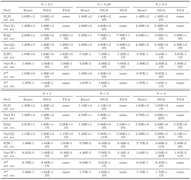
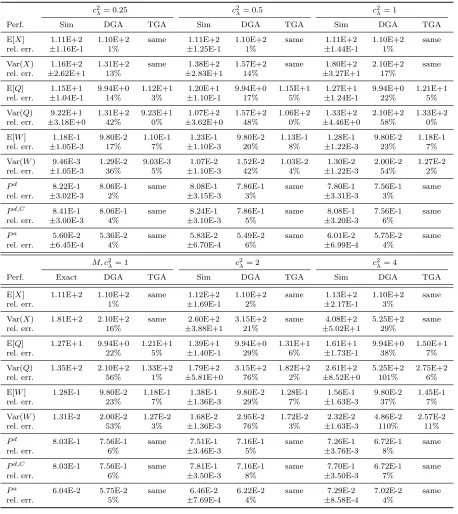
Table 3.1 A comparison of the TGA and DGA approximations to exact numerical values in the

M(λ−1)/M(1)/100 +M(θ−1) model withλ= 100ρand ρ= 1.2 for six values of θ, 0.10≤θ≤4.00. . . 43 Table 3.2 A comparison of the TGA and DGA approximations to exact numerical values in the

M(λ−1)/M(1)/100 +M(θ−1) model withλ= 100ρand ρ= 1.05 for six values of θ, 0.10≤θ≤4.00. . . 44 Table 3.3 A comparison of the TGA and DGA approximations to simulation estimates

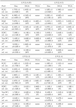
in theLN(λ−1, c2_λ)/M(1)/100 +M(2) model with i.i.d. lognormal interarrival times and (λ, ρ, θ) = (100,1.05,0.5) for six values of the interarrival time scv

c2_λ, 0.25≤c2_λ ≤4.00. . . 50 Table 3.4 A comparison of the TGA approximations to simulation estimates in the

M M P P(λ−1, c2_λ)/M/100 +M(θ−1) model with (λ, ρ, θ) = (105,1.05,0.5) for four values of the arrival process variability parameterc2_λ in (4.2), 1.5≤c2_λ ≤

10.0. . . 51 Table 3.5 A comparison of the TGA and DGA approximations to simulation estimates

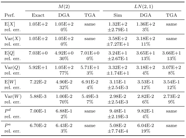
in theM/M/100 +LN(θ−1, c2_ab) model with with (λ, ρ, θ) = (100,1.05,0.5) for four values of the patience scvc2_ab, 0.25≤c2_ab≤4.00. . . 52 Table 3.6 The impact of the abandonment distribution beyond its mean and variance: a

per-formance comparison between M(λ−1₎_/M/n₊_M_{(2) and} _M₍_λ−1₎_/M/n₊_LN₍₂_,₁₎

models, where (λ, ρ, n) = (105,1.05,100). . . 53 Table 3.7 A comparison of the TGA-G, TGA and DGA approximations to simulation

estimates in the M(λ−1)/P H(1, c_s2)/100 + M(θ−1) model with (λ, ρ, θ) = (100,1.05,0.5) for four different phase-type (P h) service distributions char-acterized by their scv c2_s, 0.25≤c2_s≤4.00. . . 56 Table 3.8 A comparison of the TGA-G approximations to simulation estimates in the

M(λ−1₎_/H

2(1,2)/100+M(θ−1) model withλ= 100,ρ= 1.05 and five different

abandonment ratesθ, 0.1≤θ≤2.0. . . 57 Table 3.9 H2(λ−1,2)/P H/100 +H2(1/θ,2) with (λ, ρ, θ) = (100,1.05,0.5). . . 58

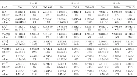
Table 3.10 Smaller scale: a comparison of the TGA-G and DGA approximations to sim-ulation estimates in the H2(λ−1)/H2(1,2)/n+H2(θ−1,2) model with three

pairs (n, ρ) withρ= 1−β/√n,λ=nρ,β=−0.5 and n= 20, 10 and 5 . . . . 60 Table 3.11 Comparison of the TGA-G and DGA approximations with theM/M/n+M(n)

approximation in [107] and simulation estimates for theM(102−1)/GI(1, c2_s)/100/200+

E2 model with four service-time cdf’s with a range of scv’s: 0.0≤c2s ≤4.0. . . 63

Table 3.12 Comparison of the TGA-G and DGA approximations with theM/M/n+M(n)

approximation in [107] and simulation estimates for theM(102−1)/GI(1, c2_s)/100/200+

(11)

Table 3.13 A comparison of TGA and DGA approximations for the probability of delay

Pd_{, the mean wait}_E_[_V_{] and the probability of abandonment}_Pa_{to the results}

in Table 3 of [94] for the M/M/n+H2 model with ρ = 1 + 1 √

n, λ = nρµ,

µ = 1 and H2 patience with (p, θ1, θ2) = (0.5,1,2). The exact results and

approximations Z&M come in [123]. . . 66 Table 3.14 A comparison of TGA and DGA approximations for the probability of delay

Pd, the mean waitE[V] and the probability of abandonmentPato the results in Table 6 of [94] for the M/M/n+H2 model with ρ = 1 + 1

√

n, λ = nρµ,

µ= 1 and H2 patience with (p, θ1, θ2) = (0.9,1,200). . . 67

Table 3.15 A comparison of TGA and DGA approximations for the probability of delay

Pd, the mean waitE[V] and the probability of abandonmentPato the results in Table 9 of [94] for the M/M/n+GI model with ρ = 1 + 1√n,λ = nρµ,

µ= 1 and increasing patience-time hazard rate. . . 67 Table 3.16 The performance for underloaded models: a comparison between simulation estimates

and exact numerical values for the M(λ−1)/M(1)/100 +M(θ−1) model with n = 100, ρ= 0.95 and 0.1≤θ≤2 . . . 69 Table 3.17 A comparison between simulation estimates and exact numerical values for the

M(102−1)/M(1)/100+M(θ−1) model, confirming the validity of both algorithms 74

Table 4.1 Evaluation of DGA and TGA onH2(λ−1(t),2)/M(1)/100 +H2(θ−1,2), where

λ(t) = 100 + 60 sint . . . 91 Table 4.2 Evaluation of DGA and TGA on H2(λ−1(t),2)/M(1)/100 +H2(2,2), where

λ(t) = 1 +csint, andc= 0.2,0.4,0.6 and 0.8 . . . 92 Table 4.3 Evaluation of DGA and TGA onLN(λ−1(t), c2_λ)/M(1)/100 +H2(2,2), where

λ(t) = 1 + 0.6 sint . . . 93 Table 4.4 Evaluation of DGA and TGA onLN(λ−1(t),2)/M(1)/100 +LN(2, c2_a), where

λ(t) = 1 + 0.6 sint . . . 94 Table 4.5 Evaluation of DGA and TGA onH2(t)/P H(1, c2s)/100+H2(2,2), whereλ(t) =

100 + 60 sint . . . 97 Table 4.6 Evaluation of DGA, TGA and TGAG in smaller systems: LN(t)/M/n +

LN(2,2) wherec2

λ = 1 and n= 50,20,10,5 and 3 . . . 98

Table 5.1 Steady-state queue length of (M+D)/(M/1)2/Π with constant pre-arrival delay119

Table A.1 A comparison of the TGA and DGA approximations to exact numerical values in theM(λ−1)/M(1)/100 +M(θ−1) model with λ= 100ρ and ρ= 1.5 for six values ofθ, 0.10≤θ≤4.00. . . 139 Table A.2 A comparison of the TGA and DGA approximations to exact numerical values

in theM(λ−1)/M(1)/100+M(θ−1) model withλ= 100ρandρ= 1.2 for three low abandonment ratesθ <0.1. . . 140 Table A.3 A comparison of the TGA-G approximations to simulation estimates in the

(12)

Table A.4 A comparison of the TGA and DGA approximations to exact values for the Markovian M(λ−1₎_/M₍₁₎_/_{100 +}_M₍_θ−1_{) model with} _n _{= 100}_{, ρ} _{= 1}_._{05 and}

θ= 4,10 . . . 143 Table A.5 A comparison of the TGA and DGA approximations to exact numerical values

in theM(λ−1)/M(1)/n+M(2) withn= 50,20,10,5,3 and 1,ρ= 1−β/√n,

λ=nρ and θ= 0.5. . . 144 Table A.6 A comparison of the TGA and DGA approximations to exact numerical values

in the M(λ−1)/M(1)/n+M(θ−1) model with (n, θ, λ) = (100,0.5,100ρ) and

ρ→1 . . . 145 Table A.7 A comparison of the TGA approximations to exact numerical values in the

M(λ−1)/M(1)/100 +M(θ−1) model with (λ, ρ) = (110,1.10) and 0.1≤θ≤4 . 146 Table A.8 A comparison of the TGA approximations to exact numerical values in the

(13)

LIST OF FIGURES

Figure 1.1 Estimated service and patience time from call centers in [15] . . . 3

Figure 2.1 An auxiliary system . . . 18 Figure 2.2 Comparison between Di(t) andSi(t) in terms of arrival times. . . 21

Figure 3.1 The relative error in the approximations of six performance measures as a function of the traffic intensity ρ for 1.001 ≤ ρ ≤ 1.500 (with ρ−1 in log scale) in the M(1/100ρ)/M(1)/100 +M(2.0) model with abandonment rate

θ= 0.5. . . 41 Figure 3.2 The relative error in the approximations of six performance measures as a

function of the traffic intensity ρ for 1.001≤ρ≤1.500 (with (with ρ−1 in log scale) in the M(1/100ρ)/M(1)/100 +M(0.5) model with abandonment rate θ= 2.0. . . 42 Figure 3.3 The relative error in the approximations of six performance measures as a

function of the abandonment rate θ for 0.01≤θ≤4.00 (with θin log scale) in the M(1/105)/M(1)/100 +M(1/θ) model having traffic intensity ρ= 1.05. 42 Figure 3.4 The relative error in the approximations of six performance measures as a

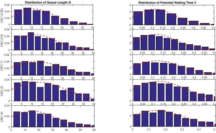
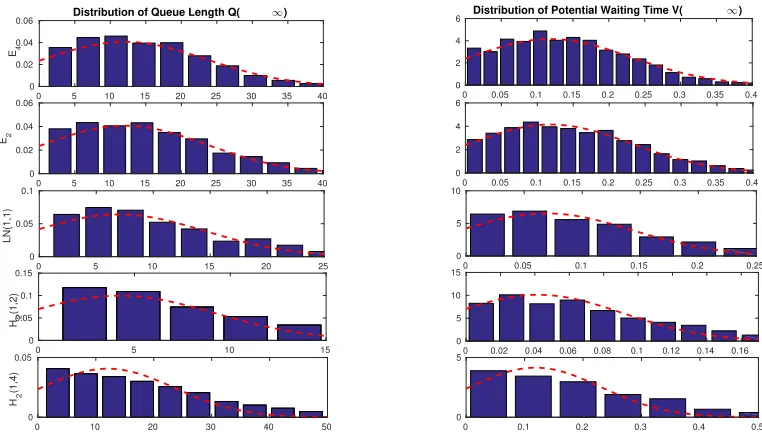
function of the interarrival-time scv c2_λ for 0.25 ≤ c2_λ ≤ 4.0 (with c2_λ in log scale) in the LN(1/105, c2_λ)/M(1)/100 +M(2) model. . . 46 Figure 3.5 Simulation estimates (histograms) of the TGA approximating distributions

of the steady-state queue lengthQn(left) and waiting timeVn(right) for the

LN(λ−1, c2_λ)/M(1)/100 +M(2) model with (λ, ρ, θ) = (100,1.05,0.5). . . 47 Figure 3.6 The relative errors in the approximations of six performance measures as a

function of the patience-time scv c2_ab for 0.25 ≤ c2_ab ≤ 4.0 (with c2_ab in log scale) in the M(1/105)/M(1)/100 +LN(2, c2_ab) model. . . 48 Figure 3.7 Simulation estimates (histograms) of the TGA approximating distributions

of the steady-state queue length Qn (left) and waiting time Vn (right) in the

M/M/100 +LN(θ−1, c2_ab) model with (λ, ρ, θ) = (100,1.05,0.5). . . 49 Figure 3.8 The relative error in the TGA-G approximations of six performance measures

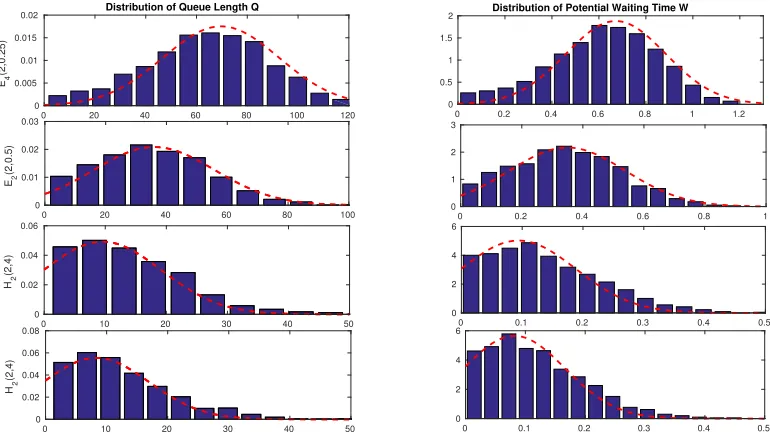
as a function of the service-time scv c2_s for 0.25 ≤ c2_s ≤ 4.0 (with c2_s in log scale) in the M(1/105)/P H(1, c2_s)/100 +M(2) model . . . 54 Figure 3.9 Simulation estimates (histograms) of the TGA-G approximating distributions

of the steady-state queue length Qn (left) and waiting time Vn (right) in the

M(105−1)/P H/100 +M(2) model for five service distributions with 0.25 ≤

c2_s≤4.0. . . 55 Figure 3.10 Simulation estimates of the relative errors in the approximations for six

performance measures as a function of the number of servers, n, for n = 5,10,20,100 (with n in log scale) in the H2(1/nρ,2)/H2(1,2)/n+H2(2,2)

model. . . 59 Figure 3.11 Simulation estimates (histograms) of the TGA-G approximating distributions

(14)

Figure 3.12 Simulation estimates of the mean and variance of the queue length as a func-tion of time in the H2/H2/n+H2 model to show the approach to steady

state. . . 71

Figure 4.1 Comparisions between queue lengths in Markovian Mt/M/s+GI model and general Gt/GI/s+GI model . . . 79

Figure 4.2 Comparisons of distributions between simulated queue lengths and DGA . . . 88

Figure 4.3 Comparison of the TGA and DGA approximations with theH2(t)/M(1)/100+ H2(2,2) model having arrival rateλ(t) = 60 sint+ 100 and SCV c2λ = 2. . . . 89

Figure 4.4 Comparison of the TGAG and DGA approximations with theH2(t)/H2(1,2)/100+ H2(2,2) model with arrival rateλ(t) = 60 sint+ 100. . . 95

Figure 5.1 Number of waiting customers with different pre-arrival Delays. . . 102

Figure 5.2 Bouncing effect in the dynamic of steady-state queue lengths for remote queue103 Figure 5.3 A remote queue with two single-server queues . . . 104

Figure 5.4 Steady-state queue lengths for remote queue having different routing proba-bilities . . . 107

Figure 5.5 The illustration of coupling . . . 113

Figure 5.6 Comparisons of remote queue performance under different policies . . . 118

Figure 5.7 Steady-state queue length comparison in (GI+D)/(GI/1)2_/_{Π under different} policy Π . . . 120

Figure 5.8 Rectangular zone on 2-D map with two servers . . . 121

Figure 5.9 The average and standard deviation of critical parameters . . . 122

(15)

Chapter 1

Introduction

This dissertation is motivated by the growing needs to improve the performance of service sys-tems, such as healthcare syssys-tems, call centers, judicial and penal syssys-tems, both front office and back-office operations in business systems and computing systems, see [1, 122, 36] and references therein. Realistic features of service systems include (i) non-Markovian probabilities structures [15], (ii) customer abandonments [20], (iii) time-varying arrivals and staffings [74] and (iv) network structures with various routing policies. All these stated features make service systems difficult to analyze exactly, therefore effective approximation techniques are needed. Approximation techniques based on heavy-traffic limits for queues systems have been proven useful since the 1930s. This dis-sertation aims to (i) advance methodology in heavy-traffic limits for steady-state queueing systems, (ii) provide useful engineering approximations for a general queueing system based on heavy-traffic limits, and (iii) develop asymptotically optimal routing policies for queueing networks.

1.1 Non-Markovian Queueing Models with Impatient Customers

1.1.1 Customer Abandonment

Customer abandonment is common in service systems: customers will often choose to leave if they have not entered service within a reasonable delay. For example, in a hospital emergency room, patients sometimes leave the hospital before being seen by doctors, known as the left-without-being-seen (LWBS) effect [122]. Meanwhile, a small number of abandonment results in significant changes in the system performance such as the customer waiting time and the waiting queue length [32, 20]. In addition, a higher level of abandonment usually indicates a lower grade of customer satisfaction. Hence the customer abandonment has been recognized as an important feature in service systems [32, 83, 123, 20].

(16)

customers in the system, probability of customer abandonment, and probability of delay. We next introduce the most basic queueing models: the Erlang models.

1.1.2 The Classic Erlang Models

Erlang models assume exponentially distributed service times for mathematical convenience. The earliest queueing model model is the Erlang-C model [24, 25], referred to as M/M/n/∞, where the first two “M”’s indicate that the interarrival times and service times are exponentially distributed, the “∞” means an infinity waiting capacity, and the “n” is the total number of servers. Customers are served in the order of their arrivals, i.e. first-come, first-served (FCFS). Customer service times are independent of interarrival times. Unlike Erlang-C, the Erlang-B model, or the

M/M/n/0 loss model, has no waiting line. So customers arriving at an M/M/n/0 system will be blocked and lost if no server is idle. Both Erlang-C and the Erlang-B models are quite tractable but restrictive, because they do not consider the customer abandonment. Later in [32], the Erlang-A model, or the M/M/n/0 +M model, was developed, where the “+M” indicates that customer patience times are exponentially distributed. Erlang-A models can be regarded as a generalization of both Erlang-B and Erlang-C models. If the abandonment rate decreases to zero, Erlang-A degen-erates to Erlang-C; if the abandonment rate increases to∞, Erlang-A becomes Erlang-B, because customers, if ever delayed, will be blocked as if they abandon immediately.

1.1.3 Non-Makorvian Models

The Erlang models are easy to analyze because the system state (such as the number of cus-tomers in the system) is a birth-and-death process, which is a special case of continuous-time Markov chain (CTMC). However, real service systems are much more complex than Markovian models. For example, statistical analysis shows that customer service times in large-scale call centers are nearly lognormally distributed and the patience times can be far from exponentially distributed, as their hazard rates are not a constant, see Figures 1.1 in [15].

There is a significant number of papers that study non-Markovian models. Whitt [107] shows that the abandonment distribution beyond its mean has a significant impact upon queueing per-formance, so the M/M/n+GI model (having a general abandonment-time distribution, i.e., the “+GI”) does not resemble the corresponding Erlang-A model. Although the service time distribu-tion beyond its mean plays a limited role when estimating mean performance measures (such as the mean waiting time) [117], we find that the service time distribution significantly affects other system performance measures (such as variances and tail probabilities of queue length, waiting time, etc.), see Chapter 3.

(17)

(a) Histogram of sevice time with mean=200, std=249 (b) Hazard rate of patience time

Figure 1.1: Estimated service and patience time from call centers in [15]

model, exact formula is not established yet. Due to the intractability of the system performance, researchers are motivated to seek approximations, many of which are based on heavy-traffic limits of queueing models, see Kingman [61, 63, 64] for theGI/GI/1 single-server model and later Iglehart and Whitt [50, 51, 108] for the GI/GI/nmulti-server queues. Halfin and Whitt later established a many-server heavy-traffic limit for the GI/M/s model in [38], which initiated a sequence of groundbreaking works on many-server heavy-traffic limits.

On the other hand, Whitt [117] developed fluid models for the stationary GI/GI/n +GI

models, and Liu and Whitt [74, 75, 76] extended the stationary fluid model to the time-varying

Gt/GI/st+GI model, having time-varying arrivals (theGt) and staffing (thest). Later in [77], Liu

and Whitt proved that a fluid model is the many-server heavy-traffic limit for the corresponding queueing models by establishingfunctional weak laws of large numbers (FWLLN) results. The fluid model provides approximations for first order performance measures such as the mean number of customers in waiting, mean waiting time, etc. Meanwhile, Liu and Whitt in [77] also established a many-server heavy-traffic limits funcational central limit theorem (FCLT) results for the time-varying Gt/M/st+GI queueing model. Their results can be used to approximate variances and

distributions of the time-varying queues having exponential service times. Based on their theoretical work in [77], we establish Gaussian based approximations for the steady-state GI/GI/n+GI

(18)

1.2 Routing to Improve Performance

Real service systems can often be modeled as queueing networks having a finite number of sta-tions. In a hospital, for instance, patients are routed among different departments such as emergency departments, operating rooms, intensive care units, etc. Patient flows and optimal routing policies in hospitals have been widely studied [27, 79, 2, 42]. However, patient flows and routing outside a hospital have not yet drawn enough attention. For instance, many hospitals start to announce their delays online, so patients can pick a less congested hospital by comparing the announced online waiting times of all hospitals. However, the actual waiting time experienced by patients may be significantly different from the announced waiting time, because the information can quick become outdated after the commute time of patients. In 2003, a Canadian lady brought her eighty-year old mother to the emergency department in Alberta, Canada. Although the announced waiting time of the emergency department was fifteen to eighteen minutes, they had to wait five hours until a doctor was available. Consequently, her mother passed away. If the delay announcements were more accurate, they could have decided to visit another less-congested hospital [88].

Motivated by health care systems, in Chapter 5 we consider a queueing network having a finite number of single-server queues in parallel. Each customer will be routed to one queue according to certain routing policies. Before actually arriving at the destined queue, each customer will experi-ence a random commute delay. We plan to device an optimal routing policy with the objective of minimizing the waiting times at all queues. Parallel queues are usually less effective than queueing models with one waiting line and a pooled service resource (i.e., number of servers) [22]. When the commute delay is close to 0, it has been proven in [95] that it is optimal to route customers using

thejoin-the-shortest-queue (JSQ) rule, which successfully synchronizes the sizes of waiting lines at

all queues when the system is in heavy traffic. Unfortunately, our simulation experiments show that JSQ performs poorly when the commute delay increases. We improve the system performance by developing a probabilistic routing policy and prove that it is asymptotically optimal as the traf-fic intensity approaches 1. In addition, we conduct simulation experiments to provide engineering confirmations. See Chapter 5 for more details.

1.3 Heavy-Traffic Limits of Queueing Models

(19)

kept fixed while the system is asymptotically in heavy traffic because the traffic intensity goes to 1. In the MSHT case, the traffic intensity is usually kept fixed while the number of servers goes to infinity. In the rest of this section, we first review the general background of weak convergence and discuss the general approach to prove weak convergence results (§1.3.1). We next review CHT and MSHT in §§??and 1.3.2.

1.3.1 Weak Convergence and Tightness

Heavy-traffic limits are often obtained through weak convergence, also called convergence in distributions. The most commonly used functional space in queueing theory is space D, which is

the space of all right-continuous functions with limits from the left. For instance, both the queue length process and the workload process can be defined as random elements in spaceD. In general,

weak convergence is defined for a sequence of probability measures in a separable metric space space

P. The weak convergence of a sequence of random elements Xn in D means the convergence of a

sequence of probability measures induced byXn,{Pn, n≥1}, to a limiting probability measure P,

if for all continuous and bounded functions f,

lim

n→∞

Z

fdPn=

Z fdP,

and we denote the weak convergencePn⇒P. See [8, 113] for more details.

Prohorov [90] developed the Prohorov metric dπ to measure the distance of two probability

measures. Specifically, for anyP1, P2∈P, the Prohorov metric is defined by

dπ(P1, P2)≡inf{ε >0 :P1(B)≤P2(Bε) +ε, for all B ⊂D},

where Bε is the open neighborhood containing B with “ε−more radius”. Mathematically, it is defined asBε≡ {Y ∈D:m(X, Y)< ε, for someX∈B}.Herem(·,·) is the metric measuring the

distance between stochastic processes in space D, and we will specify it later. See more details in

[113].

On the other hand, the convergence of Prohorov metric dπ(Pn, P) → 0 implies the weak

con-vergencePn⇒P. However, when specifying weak convergence, instead of studying the probability

measures, we often discuss random elements (such as random variables, etc.). In view of heavy-traffic limits in queueing theory, we are mainly interested in stochastic processes in space D and

spaceC, which is the space of continuous functions. Unlike the uniform metric for spaceC, elements

in space Drequire weaker metrics, such asJ1,J2 and M1 metric, see [113] for details.

There are mainly two methods to show weak convergence: one is thecontinuous mapping theorem

(CMT) and the other is the compactness approach. We review the basic version of CMT: ifXn⇒X

(20)

3.4.1-3.4.4 in [113] for extensions and more details of CMT.

Though convenient, the CMT approach sometimes is difficult to use because convenient con-tinuous functions are hard to find. So the compactness approach is usually regarded as a standard approach to prove weak convergences. The compactness approach requiresrelative compactness. A sequence of probability measures is relative compactness if and only if their closure is compact. Prohorov’s theorem [90] provided a way to relate relative compactness totightness.

Definition 1.3.1 (see §1.5 in [8]). A subset A of probability measures in space P is tight if and

only if for any ε, there exists a compact subset Kε in the corresponding funcational space such that

P(Kε)>1−ε for allP ∈A.

The Arzel`a-Ascoli theorem facilitates the developments of various tightness criterion for stochas-tic processes in spaceCwith uniform topology, and Billingsley [8] extended those results for space D. We refer interested readers to [8, 113] for details.

In Chapter 2 of this dissertation, we prove the tightness of properly scaled steady-state number for the idle servers in the GI/GI/n/0 loss model by using the definition of tightness shown in Definition 1.3.1.

1.3.2 Heavy-Traffic Regimes

Different heavy-traffic limits are obtained in different heavy-traffic regimes, which depicts how queueing parameters changes as the system scale n (the index) increases. There are two kinds of heavy-traffic regimes: convention heavy-traffic regime (CHT) and many-server heavy-traffic regime (MSHT).

CHT In CHT, the number of customers and the arrival rate λis fixed but the traffic intensity (the ratio of the arrival rate to the service rate) approaches to 1. Kingman [61, 63] studied the conventional heavy-traffic limit for the sequence of GI/GI/1 queue. In the nth GI/GI/1, there is only one server and customers follows FCFS. Customer interarrive times are i.i.d. A1, A2, . . .

with rateλandsquared coefficient variation (SCV)c2_λ. A new arrival will enter the service if there is any server idle, otherwise she will join the end of waiting queue. Their service times are i.i.d.

{Sn,i, i≥1}, having rate µn and SCV cs2. As n→ ∞, we have the traffic intensityρn ≡ _µλ_n → 1.

When the traffic intensity ρn approaches to 1, the number of customers in GI/GI/1 increases

to ∞, but the steady-state waiting time of the nth queue, denoted as Wn, is weakly convergent:

(1−ρn)Wn ⇒ W, where W is an exponential random variable having rate 2µ/(c2λ +c2s) (see [63]

for more details).

Borovhov [10] and Iglehart and Whitt [50, 51] extended the heavy-traffic limits to GI/GI/s

(21)

intensity approach 1 in the specify way:

√

n(1−ρn)→β, asn→ ∞,

where β could be any positive real number. In this regime, they showed the properly scaled total number of customers is weakly convergent to a diffusion process, i.e.n−1/2Xn(t) ⇒Xˆ(t) in space

D, given the initial condition holdsn−1/2Xn(0)⇒Xˆ(0). Here ˆX(·) is a reflected Brownian motion

with drift−βµand diffusion coefficientµ(c2_λ+c2_s).

MSHT Besides CHT, another widely used heavy-traffic regime is MSHT. In MSHT, the service rate is fixed but the arrival rate λn and the number of servers sn increases as the system index

n→ ∞ (see [48, 49] and Borovkov [11]). The way in which λn and sn increase as n → ∞ can be

arbitrary, and the most basic MSHT is to let them change proportionally, i.e., sn = n, λn = nλ.

However, in this setting, the traffic intensity ρn= λ_µ <1, so some important performance metric,

such as probability of delay, is 0. But in real practice, the probability of delay is an important metric measuring the quality of service and is not 0. Hence a more delicate MSHT is required. Halfin and Whitt in their seminal work [38] developed a new MSHT regime for the M/M/nErlang-C model and extend it to theGI/M/nmodel. The regime is later referred to as thequality-efficiency-driven

(QED) regime or Halfin-Whitt regime. In Halfin-Whitt regime, the traffic intensity ρn approaches

to 1 in a specific way as n→ ∞:

√

n(1−ρn)→β, (1.1)

where the constant β > 0 is called the quality-of-server (QoS) coefficient. Halfin and Whitt [38] showed that the properly scaled number of waiting customers is weakly convergent to a diffusion process with piecewise drift termm(x) =−µβ1{x≥0}−µ(x+β)1{x<0} and volatility 2µ. In Halfin-Whitt regime, the steady-state probability of delay is convergent to a nondegenerate probability

α(β) ∈ (0,1) and it is dependent on the QoS coefficient β. Puhalskii and Reiman [91] extended Halfin-Whitt regime toGI/P H/nand Jelenkovic et al [53] studiedGI/D/n. Reed [93] and Puhalskii and Reed [92] later generalized to queues having generally distributed service times, i.e.,GI/GI/n. Furthermore, Garnett el all. discussed the heavy-traffic limits in Halfin-Whitt regime for queues with customer abandonment (M/M/n+M) in [32]. In the presence of abandonment (the +M), the queueing model is stable when the traffic intensity ρn≥1, thus the QoS coefficient β can be

nega-tive. Mandelbaum and Zeltyn [84] later introduced Halfin-Whitt regime for theM/M/n+GImodel, having generally distributed abandonment times. Mandelbaum and Momcilovic [82] proposed dif-fusion approximations for the virtual waiting time (VWT) process and queue length process for

GI/GI/n+GI queues in Halfin-Whitt regime. Then in [19], Dai et al. studied GI/P H/n+GI

(22)

discovered the deterministic relationship between scaled abandonment process and queue length process in Halfin-Whitt regime. Kang and Ramanan [55] studied the functional law of large num-ber (fluid) limits for GI/GI/nqueue by providing a measure-valued process recording the elapsed service time for each server at present and then Kaspi and Ramana [56] extended theirs results to

GI/GI/n+GI queues which allows customer abandonment. Meanwhile, Zhang [124] also justified FWLLN limits forGI/GI/n+GI queues which proposed as fluid models in [117]. Later Kaspi and Ramanan [57] proved a functional central limit theorem of state process for GI/GI/n queues in terms of elapsed service time process as well as waiting time process.

Recently, Atar [5] studied a another heavy-traffic regime callednondegenerate-slowdown regime (NDS) which is “in the middle of” the most basic MSHT and Halfin-Whitt regime. Here “nondegenerate-slowdown” means the ratio between customer’s delay and her service time, named as slowdown, is not trivial but in the order of O(1). In the NDS regime, the joint limits of the sojourn time and service time processes were shown to be an independent reflected Ornstein-Uhlenbeck process and a “white-noise” (zero-mean) process with a size-biased mixture of exponentials as the marginal. Ward and Glynn [102, 101] and Huang et al. [41] reviewed and explored unified FCLT limits and approximations combining conventional heavy-traffic and Halfin-Whitt regimes.

1.3.3 Heavy-Traffic Limits and Gaussian Approximations

Different heavy-traffic limits are obtained in different heavy-traffic regimes. For a sequence of queueing models in a heavy-traffic regimes, the performance measure, say the queue lengthQn, is

indexed by system scalern. The heavy-traffic limits are the weak convergence limits of performance measures under different scaling. We first define the LLN-scaled performance measure ¯Qnand the

corresponding FWLLN limit Q.

¯

Qn≡

Qn

n ⇒Q,

whereQ is deterministic. Then we define the CLT-scaled performance measures ˆQn and its FCLT

limit ˆQ.

ˆ

Qn≡

Qn_√−nQ

n ⇒

ˆ

Q,

where ˆQ is stochastic. Then, the heavy-traffic limits provides the approximations to various per-formance measure of a queueing system. For example,

Qn(t)≈nQ(t) + √

nQˆ(t) +o(√n). (1.2)

In this dissertation, we aim to develop effective engineering approximations for key performance measures of the stationaryGI/GI/n+GIand the time-varyingGt/GI/st+GIqueues across a wide

(23)

[117] and Liu and Whitt [73, 75, 74, 77]. Although the queueing models they considered have a time-varying feature, which is more general than stationary systems, the established heavy-traffic limits can be applied to stationary queueing models, by setting the time-varying model parameters to constants and letting time parameter t→ ∞. MSHT FWLLN limits are deterministic approx-imations that estimate the mean of a performance measure and FCLT limits provide stochastic refinements to characterize stochastic fluctuations around FWLLN limits. However, we find that the effectiveness of approximations deteriorates when the system switches between overloaded in-tervals (OL) and underloaded inin-tervals (UL).

Based on those observations, in Chapter 3 we modified the MSHT approximations to

truncated-Guassian approximation (TGA) so that good performance prevails in a wide range of parameters.

We also extend TGA’s even further totruncated-Guassian approximation with GI service (TGAG) so that they apply the GI/GI/n +GI model having non-exponential service times. Extensive simulation works have been done to test the practical range of our approximations. In Chatper 4, we extend our techniques to time-varying Gt/M/n+GI and more generalGt/GI/n+GI queues,

and conduct various experiments to test the robustness of approximations.

In Chapter 5, we prove that parallel single-server queue under the routing policy JSQ-REB (joining-shortest-queue with root-excess bias) coincides a pooled system in a heavy-traffic regime. Specifically, we can also approximate queue length dedicated system by the heavy-traffic limit of a GI/GI/1 pooled system, which has been shown to be a reflective Brownian motion [17, 113], namely

Qn,1(t)≈Qn,2(t)≈

1 2

√

nRBM(t) +o(√n), (1.3)

where Qn,i(t) is the queue length for the ith single server in the parallel system and RM B(t) is

a reflective Brownian motion with negative drift −βµ and variabilities determined by interarrival times and service times.

1.4 Simulations

In this dissertation, an extensive amount of computer experiments simulating stochastic queue-ing systems have been conducted to evaluate the accuracy of our Gaussian approximations. All simulations are run in MATLAB.

1.4.1 Simulation Procedure

(24)

[0.95T, T] in sampling in case arrival customers occurred in the final portion has no waiting time recorded yet.

For all performance measures that we consider, we in total run R = 2,000 runs, and in each run, we collect the data evenly along the time line [0.5T, T]. In particular, in the rth simulation replication, 1≤r≤R, we periodically generate virtual arrivals at deterministic timest1, tk, . . . , tN

withtk≡k∆tand ∆t= 0.1, 1≤k≤N ≡ b0.5T /∆tc. The virtual customers arrive and abandon as

if they are the real customers but they will not be removed from the queue if they abandon. In each runr, we sample the number of customers in queue (Q), the number customers in the service (B), and head-of-line waiting time (HWT) (W). In particular, we sample the continuous-time queue-length process and number of busy servers as well as the waiting time of the head-of-line customers at discrete time pointst1, t2, . . . , tNv, and record them asQr(k),Br(k) andWr(k), while excluding

the virtual arrivals. For potential waiting time, we collect the waiting time of virtual customers since they will not leave the system even though they are noted as abandoned, denoted as Vr(k).

For probabilities of delay and abandonment, we sample indicator variables, ηd_r(k) and η_ra(k), and record 1 if the kth virtual customer is delayed or abandoned and 0 otherwise.

1.4.2 Experiments Design

A wide range of experiments is conducted to analyze the efficiency of approximations under different conditions such as abandonment rate, the number of servers (or system scales), and traffic intensity.

Customer abandonment plays a crucial role in deciding performance of stationary GI/GI/n+

GI (and time-varying Gt/GI/st+GI). As stated before, when abandonment rate is approaching

0, the model becomes a GI/GI/n (Gt/GI/st); when the rate goes to ∞, the model becomes

GI/GI/n/0 (Gt/GI/st/0), since all delayed customers will abandon immediately. Hence we evaluate

our approximations in a wide range of the abandonment rate.

In addition, all the approximations are based on MSHT limits so they should work well when the system scale is large, i.e. when the number of servers is large. However, we tested the effectiveness of our approximations in smaller systems by decreasing the number of servers from 100 to 20, 10, 5 and even 3.

(25)

1.5 Organization

In Chapter 2, we prove the tightness of diffusion scaled number of idle servers in GI/GI/n/0 loss model in Halfin-Whitt regime. In this regime, as mentioned before, the traffic intensity is scaled by the number of servers nas√n(1−ρn)→β >0, while the server rate is fixed at 1 with no loss

of generality. Little literature studies the loss model in Halfin-Whitt regime because no tractable approach is handy to analyze general GI/GI/n/0 model. In this chapter, we first construct an auxiliary system through which the number of idle servers is converted to the waiting queue length in a single-server queue, then inspired by Garmarnik and Goldberg [31], we showed the tightness of the CLT-scaled number in waiting for the single-server queue, and thus the tightness for original loss model.

In Chapter 3, we develop refined MSHT approximations for various key performance measures such as the probability of delay, mean and variance of queue length and waiting time, etc. In this chapter, we firstly obtain the steady state version of the corresponding MSHT fluid and FCLT limits based on MSHT for time-varying queueing models [77]. Then, we develop Gaussian-based performance approximation formulas for theGI/M/n+GI model. We later extend our formulas to approximate the performance of models havingGI service times by incorporating the SCV of the service times. Extensive simulations are conducted to verify the accuracy of our approximations for a wide range of model parameters.

In Chapter 4, we extend our results in Chapter 3 and develop approximation formulas of the performance measures for the time-varyingGt/M/n+GI and Gt/GI/n+GI models, such as the

mean and variance of queue length and waiting time, etc. Our time-varying formulas are developed by truncating the MSHT fluid and FCLT limits for the time-varying queueing models developed in [77]. We again conduct extensive simulations to verify the robustness of our time-varying approxi-mation formulas for a wide range of system parameters.

In Chapter 5, we study a queueing network with a finite number of single-server queues in parallel. Each customer, before arriving at a queue, has to experience a random commute delay. We first show that the commonly used JSQ policy can be disastrous to system performance and cause high system congestion. Therefore, we proposed a probabilistic JSQ policy, REB. The JSQ-REB policy combines the JSQ policy with probabilistic routing, where the routing probabilities are fine-tuned based on the system excess capacity. We proved the asymptotic optimality of JSQ-REB policy by showing that the CLT-scaled queue length process is asymptotically equivalent to that of the corresponding pooled system. Simulations are conducted to provide engineering confirmations.

1.6 Notations and Acronyms

(26)

Table 1.1: Summary of notations and acronyms

Notations and acronums Meaning

a.s. almost surely, or with probability one

Bn(·) the number of busy servers in queue

C space of continuous functions

ccdf. complementary cumulative distribution function

cdf. cumulative distribution function

CL critically loaded, or traffic intensityρn→1

CHT conventional heavy-traffic limit

CLT central limit theorem

CMT continuous mapping theorem

D space of right-continuous functions with left limits

DGA direct Gaussian approximation

EAP exogenous arrival process

ED efficiency driven

FCFS first come first served

FCLT functional central limit theorem

fdd. finite-dimensional distribution

FWLLN functional weak law of large numbers

HWT head-of-line waiting time

i.i.d independent and identically distributed

JSQ jointing-shortest-queue

JSQ-REB jointing-shortest-queue with a root-excess bais

LLN law of large numbers

MSHT many-server heavy-traffic

MMPP Markov Modulated Poisson process

OL overloaded interval

Pa

n probability of abandonment

Pnd time-averaged probability of delay

Pnd,C customer-averaged probability of delay

pdf. probability density function

(27)

Acronyms Meaning

Qn theG/G/nmany-server queue

Ql

n theG/G/n/0 loss model

Q∞n theG/G/n∞infinity-server queue

Qn(·) the number waiting customers in queue

Q(·) FWLLN limit ofQn(·)

ˆ

Q(·) FCLT limit ofQn(·)

QD quality-driven

QED quality-and-efficiency driven, i.e. Halfin-Whitt regime

ρ traffic intensity

R real line

R+ positive real line

SCV squared coefficient of variation

TGA truncatd Gaussian approximation

TGAG truncatd Gaussian approximation adapted to GI service

UL underloaded interval

VWT virtual waiting time

Vn(·) potential waiting time for queueing system

Wn(·) waiting time of the head-of-line customers in queue

Xn(·) total number of customers in the queueing model

→ almost surely convergence

(28)

Chapter 2

Tightness of Steady-State

GI/GI/n/

0 in Haflin-Whitt regime

2.1 Introduction

Markovian queueing models are mathematically tractable, but statistical analysis of real service systems reveals the service times and abandonment times are far from exponentially distributed, see Figure 1.1. However, the exact analysis for general queueing models is almost infeasible. Hence, heavy-traffic limits are developed to approximate various system performance measures. The crux to prove heavy-traffic limits is to show the weak convergence of system performance measures. The standard proof procedure is first to show prove the existence of convergent subsequences, and then to verify the uniqueness of limits for all convergent sequences. In order to show the existence of the convergent subsequences, it is suffice to show the tightness defined in Definition 1.3.1. In this paper, we aim to prove the tightness of the sequence of system performance measures.

Motivated by a theoretical work in [31] on steady-state queue length for multiserver queueing systems (GI/GI/n) in Haflin-Whitt regime, we aim to show the tightness of steady-state number of customers for loss models in the same regime. In [31], Gamarnik and Goldberg proved the tightness of steady-state queue length in the system and the corresponding large-deviation exponent. However, they did not study the tightness related to system idleness, namely the number of idle servers in the service pool. Later Goldberg [33] showed the tightness for idleness of the GI/M/n

models having exponential service time. To extend the tightness for more general queues, we firstly study the tightness of loss model. Then, according to the fact that the number of idle servers in the loss model serve as an upper bound of that in various queueing models such as GI/GI/n,

GI/GI/n+GI, etc. Thus, our tightness result for the loss model is a stepping stone for results of more general queueing models.

(29)

been widely applied in healthcare, due to the limited resources, to control the flow (and overflow) of patients requiring intensive care [71], to model ambulance deployment [96] and to determine the required number of beds, rooms and rental vehicles [21, 3] and [66].

In this chapter, we mainly study the tightness of the number of idle servers for the steady-state loss model denoted asGI/GI/n/0, which paves the way for the heavy-traffic limits of steady-state

GI/GI/n/0 loss queueing models. There has been a large body of literature on the analysis of steady-state performance measures on loss queueing models since early twentieth century, most of which mainly focuses on the analysis of probability of blocking (PoB). Erlang [25] studied the fundamental steady-stateM/M/n/0 loss model in which both interarrival times and service times are exponentially distributed. The author proposed Erlang-B function to calculate PoB. Then in

§5.7.2 in [97], the steady-state number of busy servers in theM/GI/n/0 loss model was shown to be insensitive with respect to the service-time distribution beyond its mean. Therefore, a generalization of the service-time distribution is redundant. Later progress on generalizing Erlang’s [25] work was made in by [18] and [100], by conducting the theoretical analysis for GI/M/n/0 loss models.

Notwithstanding, analytical solutions for further generalized loss model are almost intractable, and thus heavy-traffic limits are developed to estimate the system performance of loss models. Borovkov, in [11] and [12], provided rigorous basis for approximations ofGI/M/n/0 heavily loaded loss model such as Hayward’s approximations in [70]. In [104], Whitt gave a mathematical proof of Hayward’s approximation for GI/M/n/0 and further proposed effective approximations for

GI/GI/n/0 models having non-exponential service times. Whitt’s work [114], based on state-dependent analysis in the previous one [107], proposed FCLT approximations for theGI/GI/n/mn

model, where mn is the capacity of waiting room which is allowed to increase as system scale n

grows. Later in [116], Whitt gave the heavy-traffic limit for GI/H2/n/mn model having specific

hyper-2 exponentially distributed service times. In both works, the waiting room capacity mn is

required to increases as n grows, so they do not apply to the GI/GI/n/0 loss model. Recently, Li and Whitt [69] directly dealt with approximation techniques for the GI/G/n/0 loss model, by relaxing the independence assumption among service times. Their approach heavily draws on the so-calledpeakedness, that is the ratio of the variance to the mean of the steady-state number of the corresponding infinite-server model. However, the heavy-traffic limit for the loss model is still yet to established.

We focus on the loss model in Haflin-Whitt regime. Our result can help pave the way for future work on FCLT limits. The Halfin-Whitt regime, as defined in§1.3.2, though originally analyzed in [26] and [52], and formally studied in [38]. In the work of [38], the regime for multiple parallel servers with Markovian service times denotedGI/M/n, is realized by scaling both the system scalenand the traffic intensityρnin the way defined in (1.1). We can use that the traffic intensityρnapproaches

(30)

regime to queues with a mixture of exponential distributions with a mass point at 0. Mandelbaum et al. [32] and [123] studied queues in Haflin-Whitt regime with customers abandonment, in which the limiting PoD is a function ofβ ∈_R as well as the ratio between abandonment rate and processing rate.

Our contributions are twofold. First, we show that the CLT-scaled steady-state number of idle servers for the GI/GI/n/0 loss model in Halfin-Whitt regime is tight, which is not proved before. But we point out that it remains an open problem to obtain non-trivial heavy-traffic limits, and the problem is beyond the scope of this dissertation. Another contribution is the auxiliary system we construct to prove the tightness. In the auxiliary system, the number of idle servers in the loss model equal to the number of waiting customers in the single-server queue. Such a feature enables us to study more queueing models such asGI/GI/n+GI queues with impatient customers and queueing networks.

The rest of this chapter is organized as follows. We start §2.2 to prove the tightness in the loss model. We converted the problem of the loss model to a problem for a single-server queue in§2.2.1, by constructing a sequence of auxiliary systems, and we prove the tightness of for the single-server queue in § 2.2.2. We conclude this chapter in§ 2.3.

2.2 Tightness for

GI/GI/n/

0

To describe a GI/GI/n/0 loss model, we first assume two independent random variables U’s andV’s having unit mean and bounded (2 +ε)th moment, for someε >0. That is, we assume that E[A] = E[S] = 1 and E[A2+ε]<∞, E[S2+ε]<∞. We then consider a sequence of FCFSGI/GI/n/0 models under Halfin-Whitt regime, denoted as Ql

1,Ql2, . . . . In the model Qln, interarrival times

are distributed asU/λn, and service times are distributed asV, where theλnindicates interarrival

rate and we will specify it later. We define the total number of customers inQl

nasXnl(t). Initially,

we assume there are n customers in the system being served; each has the residual service time distributed as R(V) with ccdf.:

P(R(V)> x)≡

R∞

x P(V > y) dy

E[V] =

Z ∞

x

P(V > y) dy. (2.1)

In Haflin-Whitt regime, we fix that the Halfin-Whitt scalar at β > 0 and let the arrival rate

λn = n−β √

n+o(√n). We say f(x) = o(x) if f(x)/x → 0 as x increases. For convenience, we assignλn=n−β

√

nin the remaining of this chapter.

Our main result is obtained under AssumptionT0 proposed in [31], and we adopt it here.

(31)

(a) both An and Sn are non-trivial r.v.’s, that is, neither Var(A) nor Var(S) is zero, and

(b) lim sup_t→0t−1(F(t)−F(0))<∞ holds whereF(·)is the cumulative distribution function for

An and Sn, and

(c) the steady state of loss model Ql

n exists, namely, Xnl(∞)≡limt→∞Xnl(t) exists.

Remark 2.2.1. We explain the intuition of Assumption 1. Part (a) indicates that interarrival times and service times are not constant but randon variables. Part (b) means the pdf ’s of interarrival

times and service times, if exists, is finite at the origin. Such an assumption is not restrictive

because all continuous distributions and discrete distributions having zero mass at origin satisfy it. Part (c) guarantees the our discussions on steady state is meaningful, and the sufficient conditions

for Part (c) are discussed in [4].

In each loss model Ql

n, n= 1,2, . . . , we obtain the CLT-scaled steady-state number of idle

servers

ˆ

X_nl ≡ n−X l n(∞)

√

n ,

and ˆX_nl is a random variable in R. Based on Assumption 1, we give the main result.

Theorem 2.2.1. The sequence of random variables nXˆl

n, n= 1,2, . . .

o

is tight in (R,B),

where B is the Borelσ-algebra onR.

The proof consists two steps: first, we construct an auxiliary system; in the system, the number of idle servers for a loss model is equal to waiting queue length for a single-server queue. Second, we show tightness of the queue length for the single-server queue, by adopting techniques developed by Gamarnik and Goldberg in [31]. We prove the tightness according to Definition 1.3.1. Here, the compact subset K is choosed to be a closed interval [0, x] for some finite x.

2.2.1 Step I: An Auxiliary System

In this section, we construct an auxiliary system or each Ql

n, denoted as Q l,au

n . As Figure 2.1

depicts, the auxiliary system is a closed network having two stations. Such a tandem structure is initially inspired by the model used in [65]. The first station, called Station 1, is a loss model having

mn i.i.d. servers with service time distributed asS; the second station is a single-server queue with

the service time distributed as An. We set the number of servers in Station 1 to be mn satisfying

mn=

l λn

1−βn−1/2m< λn (2.2)

to make sure that Station 2 is stable and stays in Haflin-Whitt regime. We explain why mn is set

(32)

their CLT-scaled process are

ˆ

Xn,1(t)≡

mn−Xn,1(t) √

n and Xˆn,2(t)≡

Xn,2(t)−1 √

n .

The two stations shown in Figure 2.1 are fed by each other: departures from Station 1 (2) are new arrivals to Station 2 (1). Moreoever, arrivals to Station 1 might be blocked since the station does not have waiting buffer. To keep system closed, we directly send those blocked customers to Station 2. We will discuss the benefits of this feature furthermore.

1

. . .

1

.

2

Station 1 Station 2

μ

Blocked

m m-1

Figure 2.1: An auxiliary system

Initial Condition: In thenth auxiliary system, we assume there are (mn+ 1) customers in the

auxiliary system:mnof them are in Station 1 and 1 customer is in Station 2. Customers in Stations

1 have i.i.d. residual service times distributed as R(S), the same as those in Ql

n, and customers

in Station 2 has residual service time distributed as R(An). Both R(S) and R(An) are defined in

(2.1). With such an initialization, the auxiliary system depicted in Figure 2.1 has three properties as follows.

(33)

Xn,2(t) =mn+ 1, for anyt≥0.

(ii) Station 2 is always busy, i.e.Xn,2(t)≥1 for any t≥0.

(iii) The number of customers in Station 1 bounds that of the loss model Ql n, i.e.

X_nl(t)−(n−mn)≤Xn,1(t)≤Xnl(t), (2.3)

for any t≥0.

Property (i) because the auxiliary system is a closed network. The total number of customers in the system is fixed at mn+ 1. Now, after a little transformation, we find that mn−Xn,1(t) =

Xn,2(t)−1, holding for anyt≥0. That is to say, the number of idle servers in Station 1 equals the

number of waiting customers (waiting queue length) in Station 2 for any time.

Property (ii) comes from Property (i) and the structure of the auxiliary system. Because of the fact that the total number is mn+ 1 but Station 1 allows at most mn customers in it, there has

to be at least 1 customer in the Station 2, namely Station 2 is always busy. Hence, the departure process of Station 2 is an equilibrium renewal process An(t) associated with r.v.An, as the initial

service time of Station 2 is the residual service time R(An). Given that the departure process of

Station 2 is the arrival process of Station 1, the first station shares the same arrival process with those of the loss modelQl

n we built before.

Property (iii) comes from the comparison between Station 1 and loss model. For the loss model , We separate Ql

n into two service pools. The first pool has mn servers whereas the second pool

has (n−mn) servers. Customers will preferably choose the first pool, and they are served in the

second pool only if no servers idle in the first pool. In such a setting, the number of customers in the second pool is at most (n−mn), hence the number of customers is the first pool is no less than

Xl

n(t)−(n−mn)

. Therefore, the relationships in (2.3) are shown.

Given these properties of the auxiliary system, we give Lemma 2.2.1, in which the number of idle servers for a loss model (Station 1) is bounded by the waiting queue length of a single-server queue (Station 2).

Lemma 2.2.1. For any t≥0, we have

ˆ

Xn(t)≤Xˆnl(t)≤Xˆn(t) + 2β (2.4)

for any time t >0, where n−X_nl(t)≥0 is the number of idle servers in Ql

n.

Proof. For writing convenience, we drop the time t and write a≥ b to mean a(t) ≥b(t) for any

timet≥0.

(34)

Scaling both inequalities by n−1/2 provides us (2.4).

Based on Lemma 2.2.1, to show the tightness of CLT-scaled number of idle servers for a loss model, it is equivalent to show the tightness of queue length for Station 2.

2.2.2 Step II: Tightness of Queue Length for Station 2

In this section, we prove the tightness of number in waiting in Station 2, i.e., the tightness of the sequence n−1/2(Xn,2(∞)−1), n= 1,2, . . . . Here is the overview for the proof. We first bound

total contents in Station 2 by that for a (Pmn

i=1Gi)/G/1 queue, where

Pmn

i=1Gi means the arrival

process is a superposition of mn equilibrium renewal processes. Secondly, we discretize the queue

length expression for (Pmn

i=1Gi)/G/1 by adopting Gamarnik and Goldberg’s approach [31]. Then,

based on the time discretization approach, we extend the techniques in Szczotka’s proof in [99] to prove our goal.

Since Station 2 is always busy, we can regard it as the single-server queue with autonomous service, in which customers arrive according to the sum ofmn departure processes from Station 1,

see [31] and [113].

Let the sequence of interarrival time and service time on theithserver be

n R

U₁(i)

, U₂(i), U₃(i), . . . o

and

n R

V₁(i)

, V₂(i), V₃(i), . . . o

, respectively. We denote the departure process on theith server for Station 1 as Di(t). Meanwhile, we construct an equilibrium renewal process Si(t) based on the

sequence of service timeSi(t)≡max

n

n≥0 :Pn

k=1V (i) k < t

o

.

Using a coupling technique, we show that Di(t) ≤ Si(t) for all t ≥ 0. Figure 2.2 provides an

intuitive comparison betweenDi(t) andSi(t). As long as some jobs’ interarrival time is large enough

to left server idle (blank areas), the wasted utilization of server will result in fewer number finished jobs (denoted asDi(t)) than the counting process Si(t), for any timetafter black areas appear. A

rigorous proof for Di(t)≤Si(t) for anyt≥0

is given below. Rigorously, we prove Di(t)≤Si(t) for any t≥0 as follows.

Proof of Inequalify. According to the definition of couting process, we have

Di(t)≡max

(

n≥0 :

n

X

k=1

U_k(i)∨ n−1

X

k=1

V_k(i) !

+V_k(i) < t )

, (2.6)

Si(t)≡max

(

n≥0 :

n

X

k=1

V_k(i)< t )

. (2.7)

Since

Pn

k=1U (i) k ∨

Pn−1

k=1V (i) k

≥ Pn−1

k=1V (i)

k , by definitions (2.6) and (2.7), we have Si(t) ≥

(35)

Figure 2.2: Comparison between Di(t) and Si(t) in terms of arrival times.

The queue length of Station 2 is given by that of a single-server queue with autonomous service.

Xn,2(∞)−1 = sup t≥0

( _m

X

i=1

Di(t)−An(t)

)

≤sup

t≥0

( _m

X

i=1

Si(t)−An(t)

) ≤ m X i=1 sup

t≥0

Si(t)−

1

mAn(t)

,

(2.8) where the first equality holds by mathematical induction (see Corollary 1 in [31]), the second inequality holds because thatDi(t)≤Si(t) for allt≥0, and the third inequality holds by the fact

that sup{a+b} ≤sup{a}+ sup{b} for any a, b∈[−∞,∞].

Gamarnik and Goldberg [31] developed an innovative method to discretize the right-hand-side term in (2.8) so that it can be further related to the waiting time of GI/GI/1 queue. Then we prove the equivalent problem by generalizing the proof techniques given in [99]. Their discretization approach is as follows: for each i= 1,2, . . . , mn, the function sup{Si(t)−m−1An(t)} increases at

the time when Si(t) jumps, namely at kthi renewal time

Pki

l=1V (i)

l for all ki ∈ N. As sup{·} is a

continuous function, the right-hand-side term can be expressed as

m

X

i=1

sup

t≥0

Si(t)−

1

mAn(t) = m X i=1 sup

ki≥0 (

ki−

1

mAn

ki X

l=1

V_l(i) !)

.

Hence, according to Definition 1.3.1, to show the sequence of random variables

n

ˆ

Xn,2(∞), n≥1

o

is tight, it is suffice to show that for any η > 0, there exists a compact subset Kη = [0, xη] such

that

P

ˆ

Xn,2(∞)∈Kη

>1−η, for sufficient large n.

(36)

that.

P n−1/2

m

X

i=1

sup

ki≥0 (

ki−m−n1An ki X

l=1

V_l(i) !)

> x !

< η, for any n≥n0.

For convenience, we define

ζn,k = 1−

1

mn

An Vk+ k−1

X

l=1

Vl

!

−An k−1

X

l=1

Vl

!!

, (2.9)

whereζn,k’s are i.i.d. with each other. By the inequality

P

mn X

i=1

Xi> x

! ≤ mn X i=1 P Xi >

x mn

, (2.10)

we can prove Inequality (2.9) by showing

P n−1/2sup

k≥0

( _k X l=1 ζn,k ) > x ! < η mn . (2.11)

To prove Inequality 2.11, we extend the proofs of Lemma 3-5, Theorem 5 in [31] and Theorem 1 in [99]. We focus on justify the condition that guarantees (2.11) according to [31].

Proof for (2.11). We begin the proof with three preliminary Lemmas. Lemmas 2.2.2-2.2.4 below

all come from Gamarnik and Goldberg [31]. And we refer readers who are interested in proofs to Theorem 10.2 in [8], [119] (as they mentioned) and [31].

Lemma 2.2.2 (Lemma 3 in [31]). Suppose k < ∞, X1, . . . , Xk is a sequence of general random

variables,Sj =Pj_i₌₁Xi andMk= maxj≤k|Sj|. Further suppose that there exist real numbersr >2

andα >0, and a sequence of non-negative numbers u1, . . . , uk s.t. for all 0≤i≤j≤kand x >0,

P(|Sj−Si| ≥x)≤x−4α



 X

i<l≤j

ul   r 2 .

Then there exists a finite constant Kα,β, depending only on α and β, s.t. for all x >0,

P(Mk≥x)≤Kα,βx−4α



 X

0<l≤k

ul   r 2 .

Lemma 2.2.3 (Lemma 4 in [31]). For allr ≥2, there existsCr<∞(depending only on r) s.t. for

all r.v. X satisfying E[X] = 0 and E[|X|r_]_{, if} _{_X