Phase Contrast Neutron Imaging using Single and Multiple Pinhole Apertures

ABSTRACT

MISHRA, KAUSHAL KISHOR. Phase Contrast Neutron Imaging using Single and Multiple Pinhole Apertures. (Under the direction of Dr. Ayman I. Hawari (Chair) and Dr. Sujit K. Ghosh (Co-chair).)

In the present work phase contrast neutron imaging at low/medium intensity neutron sources using single and multiple pinhole apertures has been investigated. Phase contrast techniques utilize the wave nature of neutrons (along with the particle nature used by conventional neutron imaging) to enhance the material edge contrast in the object image. The technique benefits from differences in the coherent scattering length densities of different materials in the sample. The performed investigation included multiple aspects related to the theoretical understanding, simulation techniques, experimental feasibility at the PULSTAR imaging facility, and image processing/reconstruction pertaining to these techniques.

The theoretical aspects include the physical understanding of phase contrast as well as multi-pinhole imaging. The theory for the image intensity variation for mixed phase-amplitude objects was developed. Presence of an additional interaction term, quantified by the scalar product of the gradient of real and imaginary parts of the transmission function of the object, was found in the neutron intensity expression. Further, a theoretical understanding of the image formation process using multi-pinhole masks was also developed. It was shown that the formed image of the object from a multiple pinhole aperture can be written as a convolution of the source mask image at the detector with the object image obtained through a single pinhole.

Performance of phase contrast neutron imaging requires a spatially coherent beam. Spatial coherence of the beam can be increased by increasing the L d ratio and the average wavelength of the neutron beam. These methods of improving the spatial coherence lead to a significant reduction in the neutron intensity available to image the object, thereby favoring its implementation at high intensity neutron sources. However, in order to harness the potential of this technique, its usability needs to be expanded to low/medium intensity neutron sources that are more common worldwide. In the present work experimental demonstration of the technique was performed at the 1MWth PULSTAR reactor, which represents a medium intensity neutron source. This required meticulous design to maximize the spatial coherence of the beam while maintaining the neutron intensity at the image plane. Twelve inches of single crystal sapphire was used to filter out fast neutrons to lower the average energy of the neutron beam. A 500µm gadolinium foil with a 0.5mm diameter pinhole was used as the aperture following which, a 0.6o beam divergence was provided using borated polyethylene discs with holes of increasing diameter.

In order to improve the SNR in the image multiple pinhole apertures were explored. Un-coded masks were considered for this purpose. A collimator with seven pinholes was designed to perform the imaging. Masks with greater number of pinholes were studied using simulations but could not be explored experimentally due to space restrictions at the facility. The image reconstruction of the raw data was performed using a least square de-convolution technique. Tikhonov regularization was investigated in this regard to make the convolution matrices well behaved wherever required. Also, various de-noising techniques like median filtering, Wiener filtering and soft thresholding using Symlets were explored to improve the reconstructed image. It was concluded that the choice of the de-noising techniques depends upon the properties desired in the reconstructed image like smoothness, blockiness etc.

Phase Contrast Neutron Imaging using Single and Multiple Pinhole Apertures

by

Kaushal Kishor Mishra

A dissertation submitted to the Graduate Faculty of North Carolina State University

in partial fulfillment of the requirements for the degree of

Doctor of Philosophy

Nuclear Engineering Statistics

Raleigh, North Carolina 2010

APPROVED BY:

_______________________________ ______________________________

Dr. Ayman I. Hawari Dr. Sujit K. Ghosh

Committee Chair Committee Co-chair

________________________________ _______________________________

Dr. Bernard W. Wehring Dr. Jason Osborne

ii

DEDICATION

iii

BIOGRAPHY

Kaushal Kishor Mishra was born February 15th _{1981, at Bokaro Steel City, Jharkhand} India to Shri Ram Nath Mishra and Smt. Lalita Devi. Bokaro Steel City is a small place in south east of Jharkhand with an Integrated Steel Plant and a population of about one million.

In August 1999, the author began attending Indian Institute of Technology at Kanpur (IITK), India and obtained a Bachelor of Technology (B.Tech.) degree in Mechanical Engineering in May 2003. During his junior year the author came in contact with Dr. P. Munshi, a professor of nuclear engineering at IITK, and worked under him on beam hardening in computed X-ray tomography. This work made him interested in the field of Radiation Imaging.

In his senior year the author decided to continue his education by going for graduate studies in Nuclear Engineering. The author joined North Carolina State University (NCSU) as a graduate student in Nuclear Engineering in August 2003. He started in the field of Neutron Imaging under Dr. Ayman I. Hawari pursuing his interest in Radiation Imaging. The author earned his Master’s degree in Nuclear Engineering in August 2005 by designing a thermal neutron imaging facility on the PULSTAR Reactor located in the university campus. During, this period he took a few courses in Statistics and got interested in it. So, he decided to continue further for a Doctorate in Nuclear Engineering with Statistics as his co-major.

iv

ACKNOWLEDGEMENTS

The author would like to extend his deepest gratitude to Dr. Ayman I. Hawari for his guidance throughout the course of this work. He appreciates the opportunity provided to him to work with so many diligent people. The trust and the confidence shown on him by Dr. Hawari regarding this project really mean a lot to him.

The author would like to express his gratitude to Dr. Sujit K. Ghosh who agreed to spend his time and effort in guiding the author in the statistical aspects of the project. His guidance really helped the author in various aspects throughout this work. The author would also like to acknowledge the help provided by Dr. Bibhuti B. Bhattacharya. Discussions with him provided a great deal of insight to the author in various aspects related to this work.

The author expresses his thanks to Dr. Paul R. Huffman, Dr. Bernard W. Wehring and Dr. Jason Osborne for their valuable inputs and advice all throughout this work. He wants to thank all of them to serve in his committee.

The author would like to thank Mr. Andrew Cook, Mr. Larry Broussard, Mr. Kerry Kincaid, Mr. Scott Lassell, Mr. Gerald Wicks, and Mr. Stephen Bilyj for their valuable assistance in developing the Neutron Imaging Facility and performing modifications in it from time to time. He also conveys his sincere thanks to all the student operators who assisted in the facility construction and operation.

v

TABLE OF CONTENTS

LIST OF FIGURES ... ix

LIST OF TABLES ... xviii

CHAPTER 1 INTRODUCTION

... 1

1.1 Introduction to Neutron Imaging ... 1

1.1.1 History and Trends ... 2

1.1.2 Neutron vs. X-ray Imaging... 3

1.1.3 Image Formation Process ... 7

1.1.4 Detection Systems for Neutron Imaging ... 9

1.1.5 Image Degradation Sources ... 14

1.1.6 Conventional Neutron Imaging ... 18

1.1.7 Advanced Neutron Imaging Techniques ... 20

1.2 Objective ... 28

CHAPTER 2 NEUTRON IMAGING AT THE PULSTAR: AN OVERVIEW

.. 29

2.1 Introduction ... 29

2.2 The PULSTAR Reactor ... 29

2.3 Design of the Neutron Imaging Facility ... 32

2.3.1 Design Criteria and Constraints ... 32

2.3.2 Design Performance using Simulations ... 33

2.3.3 Design Verification using Simulations ... 39

vi

2.3.5 Safety and Control Systems ... 45

2.3.6 Detection Systems ... 47

2.3.7 Facility Characterization ... 55

CHAPTER 3 PRINCIPLES OF PHASE CONTRAST AND MULTI-PINHOLE

NEUTRON IMAGING

... 60

3.1 Phase contrast Neutron Imaging ... 60

3.2 Background of Phase Contrast Neutron Imaging ... 61

3.3 Motivation ... 61

3.4 The Physics of Phase Contrast Imaging ... 63

3.4.1 Kirchhoff’s Formulation ... 63

3.4.2 Fresnel Diffraction ... 65

3.4.3 Phase and Amplitude Objects ... 67

3.4.4 Non-Interferometric Phase Contrast ... 69

3.4.5 Multi-Component Systems ... 72

3.4.6 Neutron Transmission Function of Materials ... 73

3.4.7 Assumptions and Beam Requirements ... 79

3.5 Introduction to the Multi-pinhole Neutron Imaging ... 85

3.6 Image Formation using Multi-Pinhole Masks ... 88

CHAPTER 4 DESIGN AND TESTING OF PHASE CONTRAST AND

MULTI-PINHOLE NEUTRON IMAGING SYSTEMS

... 92

4.1 Introduction ... 92

4.2 Design Considerations for Phase Contrast Imaging ... 92

4.3 Image Simulation Technique ... 94

vii

4.5 Phase Image Simulations ... 102

4.5.1 Simulation Results ... 105

4.6 Design Verification and Experimental Results ... 110

4.6.1 Design Verification ... 111

4.6.2 Performance of Neutron Phase Contrast Imaging Experiments ... 116

4.6.3 Routine Performance of Phase Contrast Neutron Imaging ... 128

4.7 Design Considerations for Multi-Pinhole Collimator ... 130

4.8 Experimental Results ... 139

CHAPTER 5 MULTI-PINHOLE IMAGE RECONSTRUCTION

... 146

5.1 Introduction ... 146

5.2 Image Reconstruction: An Inverse Problem ... 146

5.3 Coded Mask Image Reconstruction ... 150

5.4 Image Reconstruction for Un-coded Masks ... 151

5.5 Simulation Results and Discussion ... 153

5.5.1 Reconstruction of the System Point Spread Function ... 154

5.5.2 Reconstruction of Simulated Test Object ... 164

5.6 System PSF Estimation and Image Reconstruction: Simulated Results ... 164

5.7 System PSF Estimation and Image Reconstruction: Experimental Results ... 177

CHAPTER 6 CONCLUSION AND FUTURE WORK

... 184

6.1 Conclusion... 184

6.2 Future Work ... 186

viii

APPENDICES

... 199

Appendix A. Fourier Transform of the Fresnel Propagator ... 200

Appendix B. Selected Properties of Fourier Transform ... 202

Appendix C. Conjugate Gradient Technique: A Brief Note ... 203

ix

LIST OF FIGURES

Figure 1.1. A comparison between neutron and X-ray attenuation coefficients [5]. ... 3

Figure 1.2. Radiograph of a computer floppy disk (a) using neutrons depicting the polymeric low ‘Z’ components clearly, (b) using X-rays depicting metallic components clearly [6]. ... 4

Figure 1.3. Schematic depicting the image formation process in conventional neutron imaging. ... 8

Figure 1.4. A characteristic curve depicting important parameters associated with it [18]. ... 11

Figure 1.5. (a) Generic shape of a PSF. (b) The normalized intensity profile of the PSF taken through its center with the depicted full width at half maximum (FWHM). ... 16

Figure 1.6. Different functional forms that can be used to model LSF and PSF. ... 16

Figure 1.7. Neutron radiograph of a spark plug at (a) 0.69nm (0.457meV) (b) 0.32nm (2.125meV). (c) Division of the two radiographs reducing the contrast of the outer steel cover [25]. ... 21

Figure 1.8. Neutron Bragg scattering edges of face centered and body centered iron [27]. ... 21

Figure 1.9. (a) Attenuation contrast image of the object obtained using particle nature of the neutrons. (b) Phase contrast image of the same object obtained using both particle and wave nature of neutrons. ... 24

Figure 1.10. The schematic of polarized neutron imaging. The spin rotation of the neutrons depends on the magnetic field along the neutron path [36]. ... 25

Figure 2.1. A picture showing the PULSTAR reactor core with all the 6 beam tubes. ... 30

Figure 2.2. The relative neutron flux profile across the PULSTAR reactor core. ... 31

Figure 2.3. Layout of the imaging facility on BT #5. ... 32

Figure 2.4. MCNP model of the PULSTAR reactor core. ... 34

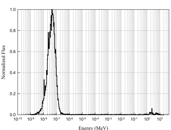
Figure 2.5. Normalized neutron energy spectrum at BT #5 entrance. ... 34

Figure 2.6. Normalized gamma energy spectrum at BT #5 entrance. ... 35

x

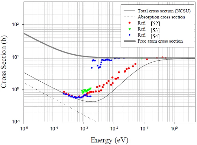
Figure 2.8. The calculated single crystal bismuth thermal neutron total cross-sections and comparison

with experimental data. ... 37

Figure 2.9. The neutron energy spectrum (dφ/d(ln(E)) at the 6m image plane with 4 inch Bi and 6 inch sapphire filters using the generated thermal neutron scattering cross-sections. ... 38

Figure 2.10. The collimator model used in the MCNP simulation. The various components that are shown in the figure are: (1) air, (2) aluminum, (3) lead, (4) SWX-277 (concrete type material with 1.6% boron content), (5) bismuth filter, (7) boral, and (8) borated polyethylene. ... 38

Figure 2.11. MCNP simulated radiograph of BPI. The pixel resolution is 50µm. ... 39

Figure 2.12. Simulated PSFs for different imaging media. ... 41

Figure 2.13. (a) Six inches long single crystal sapphire filter. (b) Four inches long bismuth filter with large monocrystals. ... 44

Figure 2.14. Photograph of the beam shutter used to open/close imaging beam. ... 45

Figure 2.15. The imaging facility shielding enclosure and the control system. ... 46

Figure 2.16. A view of the computer screen showing the safety and control system. ... 47

Figure 2.17. A picture of different equipments associated with the film detection system. ... 48

Figure 2.18. Equipments for the image plate detection system. ... 49

Figure 2.19. Thompson tube detection system. ... 51

Figure 2.20. Equipments associated with the scintillation screen detection system. ... 52

Figure 2.21. Schematic of the neutron detection within a boron doped MCP structure [66]. ... 54

Figure 2.22. The micro-channel plate detection system. ... 54

Figure 2.23. Measured neutron beam profile at the image plane located at a distance of 6m from the aperture. The pixel size is 50µm. ... 55

Figure 2.24. (a) Scanned neutron radiograph of the ASTM BPI using film. (b) Neutron radiograph of the ASTM BPI using an IP. (c) Scanned neutron radiograph of the ASTM SI using a film. (d) Neutron radiograph of the ASTM SI using an IP. ... 57

Figure 2.25. Measured LSF using a radiography film. The data was fitted to a Lorentzian function and the FWHM was extracted from the fit result. ... 58

xi

Figure 3.1. Diagram illustrating Kirchhoff's derivation of the amplitude at P due to a point source at Q. 64 Figure 3.2. Schematic for the small angle approximation of the Kirchhoff's formula. ... 66 Figure 3.3. The geometry and coordinate system for the Fresnel diffraction. ... 67 Figure 3.4. Diagram illustrating the description of wave propagation through a multi-component system. ... 73 Figure 3.5. Schematic showing the interaction of neutron with atoms leading to the creation of mean optical potential [84]. ... 75 Figure 3.6. Diagram depicting the optical path difference between the neutron waves passing through the object and the vacuum. ... 78

Figure 3.7. (a) Two monochromatic waves with a delay of τ. The coherence time τc is infinite since they are perfectly correlated with each other for all delays τ. (b) The amplitude of a wave whose phase drifts significantly in time τc as a function of time t(red) and a copy of the same wave delayed by 2τc (green).

At any particular time t the wave can interfere perfectly with its delayed copy. But, since half the time the red and green waves are in phase and half the time out of phase, when averaged over t any interference disappears at this delay [89]. ... 81 Figure 3.8. (a) A plane wave with an infinite coherence length. (b) A wave with varying wave-front and infinite coherence length. (c) A wave with varying wave-front and finite coherence length [89]. ... 82 Figure 3.9. Schematic depicting the increase in the coherence area Ac of a wave incident on a pinhole at a

large distance from the pinhole [89]. The coherence length Lc remains unchanged. ... 84

xii

Figure 4.6. Phantom 1 Simulation Results: (a) Normal Attenuation Radiograph (1st _{term in Eq. (4.9)) (b)}

The pure phase image (2nd _{term in Eq. (4.9)) (c) The phase amplitude interaction image (3}rd _{term in Eq.}

(4.9)) (d) The phase image with phase-amplitude interaction which is the difference of (b) and (c) as given by Eq. (4.9) (e) Phase contrast radiograph with pure phase approximation (1st _{and 2}nd _{term in Eq.}

(4.9)) (f) Phase contrast radiograph with phase-amplitude interaction (all terms in Eq. (4.9)). The object to detector distance R = 80cm. The grayscale for all six images is the same. ... 106 Figure 4.7. An intensity profile taken across (a) slice ‘a-a’ of Figure 4.6(e) and Figure 4.6(f) and (b) slice ‘b-b’ of Figure 4.6(e) and Figure 4.6(f). The profiles compare the pure phase and the mixed phase-amplitude approximations. The circled regions show the edge overlap effect. ... 108 Figure 4.8. The shape of the pure phase term with odd symmetry about a material edge in a sample, the phase-amplitude interaction term with even symmetry about the edge in the sample and their difference which is asymmetric about the edge. ... 109 Figure 4.9. Phantom 2 simulation results: (a) Normal Attenuation Radiograph (b) Phase contrast

radiograph with pure phase approximation (c) Phase contrast radiograph with phase-amplitude

interaction. The object to detector distance R = 50cm. ... 110 Figure 4.10. Phantom 2 Simulation Results: (a) Phase image using pure phase approximation (b) Phase-amplitude interaction image (c) The phase image with phase-Phase-amplitude interaction which is the difference of (a) and (b) as given by Eq. 4.9. The object to detector distance R = 50cm. The images were normalized between zero and one. ... 110 Figure 4.11. The divergent section of the collimator with the lead discs. The gadolinium pinhole is shown in the blowup section. The diameter of the pinhole is 0.5mm. ... 112 Figure 4.12. Alignment of the gadolinium pinhole with the lead discs using laser. ... 113 Figure 4.13. Bare beam neutron image of the gadolinium pinhole taken using image plates. (a) The raw image as obtained by reading the image plate. (b) The image processed in the multi gauge software using the spike noise filter and the 9×9 median filter. The exposure time was 60 minutes at a 6m distance between pinhole and the detector. The size of the image plate is 20×25 cm2_{. ... 114}

xiii

Figure 4.18. Plot of beam center location against the distance on the rail (which has a fixed offset from the source). Position 0 indicates the misaligned position of the rail and Position 1 indicates the corrected position. ... 119 Figure 4.19. Photograph of Sample 1 (Stack of Aluminum Plates). ... 120 Figure 4.20. Image of the aluminum stack taken (a) at R = 8cm (b) at R = 200cm. The exposure time for both of them was 120 minutes at the 1MW reactor power. ... 121 Figure 4.21. A normalized intensity profile of the top edge of the aluminum with air for Sample 1 for both the radiographs shown in Figure 4.20. Image of the aluminum stack taken (a) at R = 8cm (b) at R = 200cm. The exposure time for both of them was 120 minutes at the 1MW reactor power. The intensity clearly indicates the phase contrast intensity variation at the aluminum edge. Both the shown profile has been averaged over 400 edges to reduce the fluctuation due to noise. ... 122 Figure 4.22. Photograph of the designed phantom with the different material marked (Sample 2). ... 123 Figure 4.23. Neutron radiograph (without post processing) of Sample 2 (designed phantom) for the object-to-detector distance (a) R = 3cm and (b) R = 250cm. ... 124 Figure 4.24. Neutron radiograph of Sample 2 (designed phantom) for the object-to-detector distance (a) R

= 3cm and (b) R = 250cm. The image was de-noised using spike noise filter. ... 125 Figure 4.25. Neutron radiograph of Sample 2 (designed phantom) for the object-to-detector distance (a) R

xiv

Figure 4.33. The common illumination area at the object plane for the pinholes arranged as shown in Fig. 4.31(a) (Geometry 1). All dimensions are in centimeters. ... 136 Figure 4.34. The common illumination area at the object plane for the pinholes arranged as shown in Fig. 4.31(b) (Geometry 2). All dimensions are in centimeters. ... 137 Figure 4.35. The common illumination area at the object plane for the pinholes arranged as shown in Fig. 4.31(c) (Geometry 3). All dimensions are in centimeters. ... 138 Figure 4.36. Schematic of the diverging beam cross-section at the image plane for Geometry 3 (shown in Figure 4.31(c)). All dimensions are in centimeters. ... 139 Figure 4.37. The multi-pinhole phase contrast neutron imaging collimator design. The materials as indicated in the figure are (1) aluminum (2) borated polyethylene (3) lead (4) sapphire filter (5) SWX-277. The gadolinium mask design with the pinhole pattern is also shown in the figure. ... 140 Figure 4.38. Photograph of the manufactured multi-pinhole collimator divergent section assembly. ... 141 Figure 4.39. Bare beam image taken on an image plate placed at the farthest image plane using the multi-pinhole collimator. The exposure time is 40 minutes at 1MW reactor power... 142 Figure 4.40. Radiograph of an aluminum rod 2 inches in length 1cm in diameter taken using the multi-pinhole collimator. The object to image plane distance is 170cm. The exposure time was 120 minutes at the 1MW reactor power. ... 143 Figure 4.41. Normalized intensity profile along the edges (a) ‘a-a’ and (b) ‘b-b’ shown in Figure 4.40. 144 Figure 5.1. (a) The random multi-pinhole mask image at the image plane with 300 holes. (b) The raw image at the image plane with no noise obtained for a delta function. (c) The raw image at the image plane with no noise obtained for an inverted delta function. (d) The reconstructed delta function from Figure 5.1(b) using two-step least square de-convolution process (ε = 2.81×10−7_{± 4.73×10}-24_{). (e) The}

reconstructed inverted delta function from Figure 5.1(c) using two-step least square de-convolution process (ε = 3.84 × 10−6_{± 7.26 × 10}-22_{). All the images are in the grayscale with white being the}

xv

5.2(a) (b) Figure 5.2(b) (c) Figure 5.2(c) and (d) Figure 5.2(d). Error values of the reconstructed images from (a) to (d) are 0.122 ± 0.004 (α1= 0, α2=0.06), 0.400 ± 0.010 (α1= 0, α2=0.15), 0.680 ± 0.012 (α1=

0.1, α2=0.9) and 0.845 ± 0.011 (α1= 0.4, α2=1.4) respectively. ... 160

Figure 5.5. The surface plots depicting the variation of the error with the change in the scale parameter

1

αand α2 in the two-step regularized least square de-convolution of the images shown in (a) Figure

5.2(a) (b) Figure 5.2(b) (c) Figure 5.2(c) and (d) Figure 5.2(d). ... 161 Figure 5.6. The bar chart comparing the error values obtained in the reconstructed images using two step regularized de-convolution at optimum scale parameter values and different de-noising techniques ... 163 Figure 5.7. (a) Ideal image of the object. (b) Image of the pinhole mask at the image plane (c) The noisy raw image data at the image plane. ... 165 Figure 5.8. Reconstruction of the raw data shown in Figure 5.7(c) using (a) two-step least square de-convolution (ε = 5.061 ± 0.022) (b) two-step regularized least square de-convolution (α1= 0.2, α2= 1.7,

ε = 1.666 ± 0.003) (c) two-step regularized de-convolution followed by adaptive Wiener filtering (α1=

0.1, α2= 0.3, ε = 1.222 ± 0.003). ... 165

Figure 5.9. The MCNP model of the imaging system used to simulate the multi-pinhole images. The blow up of the Sections A is shown in Figure 5.10. ... 166 Figure 5.10. The collimator model used to perform simulation of system images. It can be compared with the designed collimator shown in Figure 4.37. The materials as indicated in the figure are (1) aluminum (2) borated polyethylene (3) lead (4) sapphire filter (5) SWX-277. ... 166 Figure 5.11. The simulated system PSF obtained using radiation transport calculations. The distance between the multi-pinhole mask and the object pinhole is 4m and the distance between the object and the image plane is 1m. The image plane grid resolution is 50µm. The image is normalized between 0 and 1. ... 168 Figure 5.12. The reconstruction of the image shown in Figure 5.11 using conjugate gradient iterative least square with no regularization. The pixel size is 50µm. The source mask image for the reconstruction was calculated using known parameters b a/ =0.25, _γ=30o _{and the source mask pinhole diameter of 0.5mm.}

... 169 Figure 5.13. The reconstruction of the image shown in Figure 5.11 using conjugate gradient iterative least square with no regularization. The pixel size is 50µm. The source mask image for the reconstruction was calculated using estimated parameters b a/ =0.243,_γ=29.99o _{and the known source mask pinhole}

xvi

image plane is 1m. The image plane grid resolution is 50µm. The image is normalized between 0 and 1. ... 172 Figure 5.15. The reconstruction of the image shown in Figure 5.14 using conjugate gradient iterative least square with no regularization. The SPSF for the reconstruction was calculated using estimated values from Figure 5.11. The pixel size is 50µm. ... 173 Figure 5.16. The reconstruction of the image shown in Figure 5.14 using conjugate gradient iterative least square with no regularization. The SPSF for the reconstruction was calculated using Figure 5.14. The pixel size is 50 µm. ... 174 Figure 5.17. The reconstruction of the image shown in Figure 5.14 using conjugate gradient iterative least square with no regularization. The SPSF for the reconstruction was calculated using Figure 5.14 with the effect of the non-zero diameter of the source mask pinholes removed. The pixel size is 50µm. ... 175 Figure 5.18. The cadmium sample used to perform MCNP simulation. ... 176 Figure 5.19. The simulated image of 1mm thick cadmium square with a rectangular hole in it. The distance between the multi-pinhole mask and the object pinhole is 4m and the distance between the object and the image plane is 1m. The image is normalized between 0 and 1. (a) The image plane grid

resolution is 50µm. (b) The image plane grid resolution is 50µm but every 4th row and column from Figure 5.19(a) is selected. ... 176 Figure 5.20. Reconstruction of the image shown in Figure 5.19(b) using conjugate gradient iterative least square with no regularization. The SPSF for the reconstruction was calculated using (a) ideal parameter values ofb a/ =0.25,_γ=30o_{, (b) parameters estimated using Figure 5.14 (b a/ =0.249,γ =30.25}o_{) (c)}

/ 0.245

b a= ,_γ=30o _{(d) b a/ =0.25, γ =31}o _{with the effect of the non-zero diameter of the source mask}

pinholes removed. ... 178 Figure 5.21. The system point spread function (SPSF) obtained using the multi-pinhole collimator. The distance between the pinhole and the detector was 130cm. The exposure time was 60 minutes at 1 MW reactor power. The image has been normalized between 0 and 1. ... 179 Figure 5.22. De-noised SPSF using (a) 7×7 Median filtering. (b) 7×7 Wiener filtering (c) soft

thresholding of Symlet (of order 4) coefficients using a threshold of 0.3906. The SNR for these images are 21.98, 22.95, and 18.41 respectively. ... 180 Figure 5.23. Reconstruction of the image shown in Figure 5.22(b) using conjugate gradient iterative least square with no regularization. The SPSF for the reconstruction was calculated using parameter values ofb a/ =0.237, _γ=14.5o_{. ... 182}

xvii

xviii

LIST OF TABLES

Table 1.1. Performance parameters of different neutron detection systems for imaging purposes under the

condition at the radiography station NEUTRA at PSI [17]. ... 10

Table 2.1. Final parameters of the designed neutron imaging facility. ... 40

Table 2.2 Grades of single crystal sapphire [47]. ... 43

Table 2.3 Measured beam parameters according to ASTM (E-545) standard. The 3rd _{column has} parameters calculated using an IP image even though it is not prescribed by the ASTM. ... 56

Table 3.1 The list of various facilities where phase contrast neutron imaging has been performed. ... 62

Table 4.1 The material composition of the phantoms used in the simulations. ... 104

1

CHAPTER 1

INTRODUCTION

Radiation imaging has been a well known technique for non-destructive testing (NDT) and non-invasive measurements (NIM) of materials. Almost all different kinds of radiations like photons, gamma rays, X-rays, electrons, neutrons, micro waves, radio waves etc. are used for obtaining multitude of information about an object non-destructively, by performing a transmission or reflection imaging of it. The use of these different kinds of radiation particles is associated with certain advantages and limitations. Therefore, depending upon the type of sample and the objective of imaging exercise, the suitability of the type of imaging can be decided. In the present case the focus is on imaging with neutrons. Specifically, non-interferometric phase contrast imaging was investigated in this work.

In the present Chapter an introduction to neutron imaging is being presented. This includes its usefulness as a radiation imaging technique, the process of image formation, the detection systems used, the different neutron imaging techniques and the process of image degradation. Finally, the purpose and motivation of the present work will be outlined in the last Section of this Chapter.

1.1

Introduction to Neutron Imaging

2

different than X-ray or gamma-ray attenuation characteristics for any object, results into an image formed that depicts different information about the object.

1.1.1 History and Trends

Radiography with neutrons began shortly after the discovery of neutrons in 1932 by James Chadwick. The initial experiments in neutron radiography were performed in Germany in the late 1930’s by H. Kallmann and E. Khun [1]. In the years 1935 to 1938 H. Kallmann and Khun used Radium-Beryllium (Ra-Be) sources and a small neutron generator at the research laboratory of the I.G. Farben Aktiengesellschaft to develop methods of photographic detection of neutrons. The findings of the study by Kallmann and Khun got published several years after the work was finishedand reported in several patents conclusively showing the potential of neutron radiography. However, the available neutron intensities were insufficient for practical industrial neutron radiography, and it was not until after the work of Fermi and co-workers on the thermal neutron reactor that, in 1955, the first neutron radiographs were taken using a reactor beam (8 MW BEPO reactor at Harwell) [2]. In 1960s and 70s the popularity of neutron radiography increased at other places with the help of people like J. P. Barton, Harold Watts, Dan Polanski, Harold Berger etc. It got further momentum with the formation of the Neutron Radiography Working Group (NRWG) in 1979 which lead to a coordinated effort and promulgation of knowledge in a systematic manner within the community [3]. In 1981, the First World Conference on Neutron Radiography was held in San Diego, California, USA. The formalization of this existing worldwide community of scientists into the International Society of Neutron Radiology (ISNR) started in 1992 [4].

3

1.1.2 Neutron vs. X-ray Imaging

Often neutron imaging is considered as being complimentary to X-ray or gamma-ray imaging. Figure 1.1 presents a comparison between neutron and X-ray attenuation for different elements [5]. From the figure it can be clearly observed that the neutron attenuation and hence its cross section does not follow a particular trend with the atomic number (Z) of the elements.

Figure 1.1. A comparison between neutron and X-ray attenuation coefficients [5].

4

compounds like different kind of polymers, organic materials etc. can provide higher contrast in the neutron image. As an example, the neutron and X-ray radiograph of a computer floppy disk is shown in Figure 1.2 [6]. The neutron radiograph clearly depicts the polymeric components of the floppy disk where as X-ray provides more contrast for the metallic components. This is a good visual description indicating the complementary nature of the neutron and X-ray imaging. This complimentary nature can be utilized fruitfully in the NDT of various objects to a large degree.

Figure 1.2. Radiograph of a computer floppy disk (a) using neutrons depicting the polymeric low ‘Z’ components clearly, (b) using X-rays depicting metallic components clearly [6].

5

becomes possible to locate the defects which may not become visible in the regular neutron or X-ray image.

But despite the advantages which neutron imaging offers over photons (γ- and X-rays) it also has some difficulties associated with it. The first difficulty associated with neutron imaging is the limited availability of high flux neutron sources for such applications. Also, often the neutron beam obtained from such sources is contaminated with gamma rays. In the case of photons the sources can be obtained or manufactured (X-rays) easily with required flux and are also not very expensive. In the case of neutrons the available sources can be divided into three types: [7]

• Reactor source

• Accelerator-based sources

• Radioactive sources

Cost wise, these sources (except radioactive sources which have the least neutron flux comparatively) are significantly more expensive than photon sources. Also, the physical size of these sources is much larger than the same flux or even a much higher flux gamma ray or X-ray source. Thus, portability of such sources is less.

Other problem associated with neutron source is “thermalization” of the neutron beam. Neutrons are mainly categorized based on their energy into five categories [7]:

• Cold Neutrons (below 0.01 eV)

• Thermal Neutrons ( 0.01 to 0.3 eV)

• Epithermal Neutrons (0.3 to 10,000 eV)

• Fast Neutrons (10 keV to 20 MeV)

6

Neutron imaging is performed mainly in the thermal and cold region due to the large cross section for attenuation and detection in this energy range. Advantages of neutron imaging mentioned above are applicable for thermal and cold neutron beams. Therefore, fast neutrons generated from the source must be moderated (lowered in energy) by some means. Usually hydrogenous material (e.g., water) or graphite is used for this purpose. But this tends to increase the size of the sources and hence decrease their portability further.

The third difficulty associated with it arises from one of its advantages only, i.e. to be able to image hydrogen contain materials. Cold and thermal neutrons that are often used for performing imaging have very high scattering cross-section for hydrogen. Although this helps in detecting presence of hydrogen in the sample, it does not take a lot of it to saturate the image. Therefore, differentiation between different hydrogenous materials may not be possible even when the samples are reasonably thin. Moreover, other features of the sample may get overshadowed by the very high contrast produced by hydrogen in the sample. Similarly, some other materials like cadmium, boron, gadolinium etc., due to their high absorption cross section, can also be traced using neutrons if present in very small quantities but, their presence in somewhat larger quantities can easily stop the neutron from penetrating the sample leading to a loss of contrast available for other materials present in the object.

The fourth difficulty associated with neutron imaging is related with the detection technique. In the case of photons the image can be directly taken on a film. But neutrons will not form image directly on a film. Hence, some mechanism is required which converts the neutron signal into a detectable secondary radiation signal without adding much noise or without reducing the signal strength appreciably. For this purpose a converter screen (intensifying screen) is used which in principle absorbs the neutrons and emits photons or electrons to which the image recorder is sensitive. This extra process makes the detection efficiency of neutron less than the gamma rays for similar detectors and also adds to the image unsharpness. Further, it requires the beam to have high neutron-to-gamma (N/G) ratio as the gamma rays will also get detected on the detector with an equal or lesser efficiency depending upon the type of detector being used.

7

associated with the neutrons. The quality factor for neutrons is 20 times more than that of photons [8]. Therefore, neutrons are potentially more damaging to human tissue than photons. Moreover, the presence of sufficient number of fast neutrons in the neutron beam even after the process of thermalization and filtering can make the shielding problem more difficult to handle than photons. The thickness of the shielding can be as large as a three to four feet consisting of stacks of various neutron and photon attenuating materials. When there is a constraint on the available beam-line space then a good design of shielding fulfilling the dose requirements while taking as little a space as possible can be an elaborate problem.

But there are some applications where neutron imaging is the only feasible option for the NDT. One example is the inspection of radioactive materials, a problem which is becoming more prevalent in this nuclear age. The radioactivity of the inspection sample can present problems for conventional radiographic methods because the X-ray films are fogged by the radioactive decay radiation from the sample. For this a special neutron radiographic technique, called the transfer detection method can be used [7]. Additional types of applications become obvious when one appreciates that significant neutron-attenuation differences often occur between isotopes of the same element [9]. Useful neutron radiographic work in this area has included differentiation between Cd113 _{and other cadmium isotopes in an irradiated reactor} control element [10] and between isotopes of uranium. Also, the difference between neutron cross-section of hydrogen and deuterium is used to establish the contrast matching concentration in biological analysis of tissues. There are various other applications like imaging of fuel cells, biological materials, reactor fuel rod cladding, plant tissues etc. where neutron imaging has been used to perform NDT/NIM of low ‘Z’ materials which do not produce enough contrast with X-rays [11]-[14].

1.1.3 Image Formation Process

8

respectively whereas ψt

( )

x y, denotes the secondary radiation profile at the image plane induced by the neutrons on the converter material. Characteristics of the neutrons being emitted by the neutron source are modified in the collimator in order to meet the desired qualities in terms of its energy spectrum, directional properties and N/G ratio while maintaining sufficient neutron flux intensity at the image plane. These qualities of the neutron beam are achieved by proper design of different elements of the collimator like beam filters, aperture, divergence angle etc. Neutrons with these desired properties being emitted through the collimator get attenuated in the sample. The attenuated neutron beam falls on the convertor screen which emits secondary radiation proportional to the neutron intensity. This secondary radiation is capable of producing an image on the recorder which could be a photographic film in some practical applications.

Figure 1.3. Schematic depicting the image formation process in conventional neutron imaging.

The whole image formation process can be illustrated by the sequence of physical transformations shown in Eq. (1.1). In the equation, D x y

( )

, represents the optical density or the gray scale density distribution that develops on the recorder (photographic film or digital media) when it is exposed to the secondary radiation ψt

(

x y t, ,

)

.

)

,

(

)

,

(

)

,

(

)

,

(

η

ζ

→

φ

t

u

v

→

ψ

x

y

→

D

x

y

9

1.1.4 Detection Systems for Neutron Imaging

Various different kinds of detector systems (convertor + recorder system) are available with different characteristics to record the neutron image. Some of the available choices are photographic films with an intensifying screen, track etch detectors, digital image plates, scintillation screens with CCD, micro channel plates, silicon flat panel screens, Thompson tubes etc. Traditionally, photographic films with intensifying screens have been used as the detector for neutron imaging. There are three basic types of intensifying screens available to be used with films - granular or crystalline, glass, and foil, in order of increasing resolution and decreasing speed (sensitivity to neutrons (explained later in detail)). In the past, some of the exclusively used screens in these categories for practical work are NE 421- granular, NE 905- glass, Gadolinium (Gd) - foil, Dysprosium - foil [15]. Even currently, for routine NDT applications films with Gd intensifying screens are the choice for the recording media. American Society of Testing and Materials (ASTM) has defined standards for performing neutron imaging for only film detection system [16]. This is because, film still has higher spatial resolution than most of the other options available even though it is one of the oldest and simple to use detection methods. Moreover, film detectors can be made in large sizes to image large samples. Table 1.1 compares the performance characteristics of some of the available detection systems under the conditions at NEUTRA facility [17]. From the table it can be clearly observed that film has a spatial resolution range between ~20µm to ~50µm. The only other detector which compares with the film are the track etch foils made up of dielectrics like glass, mica, plastics etc. where, the tracks caused in them by the radiation damage are chemically etched in a preferential manner so that the tracks become visible. A collection of many tracks form the visual image of the object. The drawbacks associated with the film detection system are the small dynamic range, no time resolution and high gamma sensitivity. Other detection systems like digital image plates, scintillation screens etc. have been developed in the last two decades which perform better than the film system in terms of these characteristics.

10

Table 1.1. Performance parameters of different neutron detection systems for imaging purposes under the condition at the radiography station NEUTRA at PSI [17].

Detector

System X-ray film and Transmission light scanner

Scintillator +

CCD camera Imaging Plates Amorphous Silicon Flat Panel

CMOS pixel detector

Max. spatial

resolution (µm) 20-50 100-500 25-100 127-750 200 Typical

exposure time for suitable image

5 min. 10 sec. 20 sec. 1-10 sec. 0.1-50 sec.

Detector Area

(typical) 18cm × 24cm 25cm × 25cm 20cm ×40cm 30cm × 40cm 3.5cm × 8cm Number of

pixels per line 4000 1000 6000 1750 400 Dynamic Range 102 _{(Non-linear) 10}5 _{(Linear) 10}5 _{(Linear) 10}3

(Non-linear) 10

5 _(Linear)

Digital format 8 bit 16 bit 16 bit 12 bit 16 bit Readout time 20 min. 2-100 sec. 5 min. 0.03-1 sec. 0.2 sec.

density D x y

( )

, , where, the exposure E x y

( )

, of the recorder at an arbitrary point

( )

x y, on the image plane is defined as the integration of the secondary radiation flux ψt

(

x y t, ,

)

(considering ψt as time dependent) over exposure time τE. The characteristic curve shape

depends upon the type of the recorder, the exposure time τE, the type of secondary radiation

11

which is directly proportional to the amount of exposure or else the precise characteristic curve should be known. But in no situation it should be allowed to saturate, because after that optical density becomes constant and hence no differentiation can be achieved between different exposures of the recorder due to varying neutron attenuation in the different regions of the sample.

Figure 1.4. A characteristic curve depicting important parameters associated with it [18].

For most of the digital detection systems the dynamic range is larger than that of films. For digital image plates and scintillation screen with CCD system the dynamic range is more than 100 times larger than the film (refer to Table 1.1) [17]. Further, the linearity within this range is also greater for these detection systems than that of film. Thus, in the case of film the exposure time should be carefully selected in order to keep the film response within the dynamic range which is not much of a problem for the digital detection techniques.

12

the time resolution of the detection system. The efficiency of the detection system is dictated by the conversion screen material, its thickness and the neutron energy spectrum. The screen efficiency ε

( )

E can be defined by

( )

{

( )

}

( ) ( )

0

exp

t

E E x E R x dx

ε =

_∫

−Σ Σ (1.2)

where, t is the thickness of the screen, Σ

( )

E is the energy dependent macroscopic neutron absorption cross-section of the screen material and R x

( )

describes the attenuation of the secondary radiation in the screen material. If the neutron energy spectrum is known then the average efficiency εavg can be calculated as

( ) ( )

( )

max max 0 0 E avg E

E E dE

E dE ε φ ε φ =

∫

∫

(1.3)

where, φ

( )

E is the neutron flux energy spectrum and Emax is the maximum neutron energy in

the energy spectrum. It can be easily observed that to obtain the higher neutron conversion efficiency the conversion screen should have high macroscopic absorption cross-section with an optimum thickness to absorb most of the neutrons. The thickness is limited by the attenuation of the secondary radiation produced due to absorption of neutrons, which is not desirable. High efficiency is a key in decreasing the exposure time required by the detector thereby improving the time resolution.

13

required per pixel to obtain the desired gray scale density on the recorder is less. This helps in decreasing the exposure time for a fixed neutron flux and average efficiency. It also helps in performing neutron imaging with low neutron fluxes without making the exposure time too long. This makes high sensitivity detectors very desirable for performing some imaging exercises like real-time neutron imaging, phase contrast neutron imaging etc. But, the images obtained with the high sensitivity detectors tend to have more noise in them because the detector captures the random fluctuations in the neutron beam. Because of the high time resolution of the detector the random fluctuations get less time to average out over time. Therefore, usually as the detector speed increases the spatial resolution decreases.

14

of the film detection system. They have higher time resolution because of less attenuation of the secondary radiation (which is conversion electrons) before being trapped in the storage phosphor. Moreover, they have lower spatial resolution which increases their speed by providing larger number of neutrons per pixel thereby reducing the exposure time. But, in high gamma content beam even the image plates will not perform satisfactorily. It has been studied that for Fuji’s BAS-IP ND-2025 (which are often used image plates) a gamma dose rate of 1µS/h is equivalent to a neutron flux of about 1.2n/cm2_{.sec [19]. To enhance the gamma} rejection capability of the neutron IPs alternative conversion materials like Li6_{F with storage} phosphor like KCl:Eu2+ _{and KBr:Eu}2+ _{have been proposed [19]. But, this leads to an increase in} the thickness of the recording layer of the IPs and a decrease in their spatial resolution. Even with this tradeoff under unavoidable conditions of high gamma background the high gamma rejection capability may be a desirable characteristic.

This makes the ratio of neutron to gamma sensitivity an important property to be considered in selecting the detector type. If this ratio is not sufficiently high then care should be taken in the design of the collimator to maximize the N/G ratio thereby minimizing the gamma exposure of the detector while taking the images. That is why for the use of photographic film as the imaging medium the N/G ratio of the beam should be kept considerably large. For this reason N/G ratio is one of the parameters in defining the beam quality using ASTM standards. But, in some imaging modalities like pinhole imaging, phase contrast imaging where pinhole neutron sources are desired, maintaining a large N/G ratio can turn out to be challenging. In such circumstances detectors with high neutron to gamma sensitivity that are less affected by the gamma rays during their exposure like digital image plates can be used to perform imaging.

1.1.5 Image Degradation Sources

15

detection system. Also, it relates to the visual image quality of the obtained radiograph which is mostly degraded by the noise sources.

The image formed using the process of neutron imaging is degraded due to multiple sources of degradation involved in the formation process which are dependent on the system geometry during the imaging exercise, the object characteristics, and the detection system characteristics. The sources of degradation can be broadly classified into two categories namely: the Blurring Sources and the Noise Sources. The blurring sources contribute to the point spread function (PSF) of the system making its spread larger, thereby blurring the image that results into unsharp edges. The PSF of the imaging system is the image of a point object taken with the system. This is also sometimes referred to as the Impulse Response of the system. Usually, the measurement of the system PSF (independent of the object being imaged) is performed by imaging of a pinhole that is materialized using neutron absorbing materials like cadmium or gadolinium with a small hole in it. A typical intensity profile of such a radiograph is shown in Figure 1.5(a). To quantify the spatial resolution of the system the full width at the half maximum (FWHM) of the intensity profile going through the center of the PSF, as shown in Figure 1.5(b), is taken most of the time [20]. This indicates the resolution of the system for an ideal neutron absorbing object. For other kind of objects that scatter neutrons the resolution will be worse than this. Sometimes, instead of measuring the PSF, an edge spread function (ESF) is measured using a sharp edge, again made up of a neutron absorbing material. The profile of an edge spread function looks like an edge function with some spread. That curve is then differentiated in order to obtain the line spread function (LSF) profile that looks similar to the profile shown in Figure 1.5(b). FWHM can be calculated from the LSF can be also used to define system resolution. The LSF is basically a PSF integrated over a line. Therefore, the spatial resolution obtained from the FWHM measurement of the LSF is a little larger than the PSF FWHM ideally. But, since in experiments, pinholes used to measure PSF always have non-zero diameter so the difference between spatial resolutions obtained using PSF and LSF may not be significant enough to observe.

16

by an inverse tangent function with additive and multiplicative parameters for scaling and shifting of the function. Different functional forms which can be used to model LSF/PSF are shown in Figure 1.6. Often either Lorentzian or a Gaussian function with scale and shift parameters are used as the exponential function is not smooth at the maximum [21]. Various different sources that contribute to the spread of PSF or the blurring are geometric, recorder, converter and the motion of the sample relative to the system.

(a) (b)

Figure 1.5. (a) Generic shape of a PSF. (b) The normalized intensity profile of the PSF taken through its center with the depicted full width at half maximum (FWHM).

17

The geometric blurring takes place due to the spread of the neutron source and depends upon the sample-to-detector distance R as well as the L d ratio of the system where L isthe source-to-sample distance and d is the effective diameter of the neutron aperture which decides the source size being observed by the object. The blur increases with increasing R and decreasing L d.ratio. Therefore, lower beam divergence or larger L d ratio is always desirable. Also, often the sample is either kept in contact with the film or very close to it in order to minimize the geometric unsharpness in the image. Still, for bigger samples the regions far from the image plane can have significantly greater geometric blurring than the regions close to the image plane. In such situation either the L d ratio of the system should be increased or image post processing may be performed to de-blur those regions selectively. There are some techniques where sharp images are produced even when the distance R is large. The sharpness comes from very high L d ratio in such systems and is also related to one of the alternative contrast enhancement mechanisms demonstrated using neutrons recently- the phase contrast mechanism.

Recorder and convertor unsharpness pertains to the detection system being used. For the film system it depends on the size of the silver halide particles, the distance between the convertor and the recorder and the thickness of the convertor. For digital image plates, along with these factors, the size of each pixel as well as the spread of the laser beam which reads the image plate also contributes to the unsharpness. Similarly, for scintillation screen and CCD systems the pixel size of the CCD as well as inaccuracy in the optics will be the additional factors contributing to the unsharpness of the image. The motion unsharpness is present only when there is a relative motion between the sample, the source and the detector. This can happen due to unnecessary vibrations present from some sources or due to motion of the sample in case of real-time imaging. To remove the unsharpness from the image various de-blurring techniques can be used. A few of these techniques will be discussed in detail in the later chapters.

18

these noises the design should be performed to maximize the N/G ratio and minimize the scattering of neutrons. To maximize the N/G ratio various gamma filters like lead, bismuth etc can be used. To minimize the scattering the shield walls could be made to absorb more neutrons and scatter less. Also, helium filled collimator can be used to reduce the scattering noise. Less scatter loss also leads to a gain in the neutron intensity at the image plane which helps in improving the signal to noise ratio (SNR). As a rule of thumb for thermal neutrons there is a 10% gain in the intensity per meter of helium compared to air [22]. The noise in the image is also related to the exposure time and the beam intensity per pixel of the detector. As the pixel size decreases, to obtain better spatial resolution, the neutrons available per pixel per unit time reduces, which leads to more statistical fluctuations. Similarly, when the exposure time is decreased, a higher standard deviation of the gray scale intensity is observed due to fluctuations in the beam. In these cases frame averaging is usually performed to reduce the fluctuations. Image de-noising methods can also be used to de-noise the images. Some of these techniques will be discussed in the later chapters.

Thus, the image data collected is a superposition of the ideal object image with the local point spread function and the noise. This, kind of image degradation happens in almost any kind of imaging. The difference lies in the sources of degradation and its mechanism whose understanding leads to its treatment thereby restoring the image. Plenty of work has been performed in the field of characterizing and restoring images obtained from radiation imaging or visual imaging. Some of the references that are relevant and are directly related to blurring mechanisms in radiation imaging are [20], [21], [23]-[25].

1.1.6 Conventional Neutron Imaging

19

material composition and thickness. The use of contrast agents mentioned above to increase the attenuation at desired places like cracks, voids, etc. in the sample in order to obtain higher contrast at those locations in the image widened its scope further to a wide variety of NDT applications in different materials. This is the contrast mechanism that is used in the conventional neutron imaging. Such imaging exercise is usually performed using a time continuous thermal neutron beam having a distribution of energy. The object is placed close to the neutron detector and the obtained image is averaged over the neutron energy spectrum, the object thickness and the exposure time. Thus, conventional imaging does not impose stringent requirements on the neutron beam energy, timing and directional characteristics to perform the imaging which makes it simple to implement, standardize and use for different imaging applications. It has been used to perform practical neutron imaging for NDT purposes over many years and has turned out to be quite successful as an NDT technique with the use of contrast agents and transfer technique. It has been routinely used to perform NDT of turbine blades, nuclear fuel pins, honeycomb structures etc.

20

unreasonably low levels other novel approaches have been proposed and demonstrated. These techniques necessarily require post processing of the collected raw image data in order to obtain the desired image and will be discussed in later chapters.

1.1.7 Advanced Neutron Imaging Techniques

As mentioned before, conventional neutron radiography uses attenuation contrast mechanism to generate contrast in the image. This may not provide enough contrast in the image for some objects. For an improvement in the contrast resolution alternative mechanism has to be utilized along with this. Some imaging techniques have been demonstrated which can generate more contrast in the images of such objects utilizing the attenuation contrast mechanism in a different way by specifically controlling the beam characteristics or by using a different contrast mechanism altogether. These techniques will be referred to as advanced neutron imaging techniques.

1.1.7.1 Energy Selective Neutron Imaging

Conventional neutron imaging works in the ‘integrating mode’ in which the image captured is averaged over the full applied energy spectrum. In the last few years energy selective neutron imaging methods have been demonstrated using thermal and cold neutrons which offer higher contrast images for the sample if the energies of the neutrons are selected correctly. As an example Figure 1.7(a) and (b) show the neutron radiographs of a steel plug taken at two different wavelengths (0.69nm (0.457meV) and 0.32nm (2.125meV)) having almost same attenuation coefficient for steel. When these two images are divided (as shown in Figure 1.7(c)) then the outer steel cover is reduced in contrast making the internal features more clear [26].

21

coherent elastic scattering or the Bragg scattering results in the appearance of these Bragg edges. Bragg edges are most pronounced and best separated in the cold followed by the thermal neutron energy ranges. The lowest Bragg edge corresponding to the largest spacing lattice planes is called the Bragg cut-off. For many engineering type materials such as iron, copper, zirconium, aluminum etc. the Bragg cut off occurs at the thermal to cold neutron wavelength of about 0.4nm (1.4 meV) [27].

Figure 1.7. Neutron radiograph of a spark plug at (a) 0.69nm (0.457meV) (b) 0.32nm (2.125meV). (c) Division of the two radiographs reducing the contrast of the outer steel cover [25].

22

It should be noted that energy selective neutron imaging does not offer any extra advantage for the neutron absorbing materials. But, often for practical thermal and cold neutron imaging, neutron absorption plays a minor role compared to the scattering except for materials like cadmium, boron, gadolinium etc. In transmission neutron imaging all neutrons that interact with the sample and do not reach to the detector, i.e. are removed from the primary beam are attributed to the total attenuation coefficient (macroscopic cross-section) given by

(

)

1 i i n

tot i s a

i

N σ σ

=

Σ =

∑

+ , where Ni is the atomic number density and σi (s = scattering, a =

absorption) is the microscopic cross-sections of the ith _{isotope component. The absorption} cross-section has generally a simple linear dependence in the cold and thermal neutron energy range. The scattering cross-section contains contribution from the Bragg, incoherent, small angle, and inelastic scattering. The captured image, as explained earlier, is given by

( )

(

) ( )

( , , , )

, , , tot x y z E dz

o

I x y =

∫

I x y E ε E e∫Σ dE, (1.4)

where I x y Eo

(

, ,

)

is the spatial energy distribution of the initial beam intensity, ε

( )

E is the energy dependent efficiency of the detection system and z is the direction of propagation of the neutron beam. Equation (1.4) assumes the validity of the exponential attenuation (Beer- Lamberts law) which is true only in the first order. The inversion of Eq. (1.4) can be performed to obtain the material cross-section information if the thickness of the material is known. This process of inversion gets simplified if the energy spread of the neutron spectrum is reduced to a very small value. Moreover, if the mean energy is made to coincide with one of the Bragg edges of the material, which are discontinuous jumps in the material cross-section (see Figure 1.8), then the inversion can lead to very accurate material composition information. The texture of the material can also be obtained through this if R

( )

β_hkl , which is the ratio of the number of crystallites in the Debye-Scherrer cone of the textured material to the corresponding number for a perfectly random sample, is included in the inversion process [27].

23

beam where λ is the wavelength of the beam and ∆λ is the spread in the wavelength of the beam. There are several ways in which this is achieved in the cold energy range [28]:

• With a turbine type energy selector (chopper) – the velocity and the tilting angle are used to select the energy band. Most of the turbine selectors provide an energy resolution of ∆λ λ~ 10% or higher [27].

• With a single crystal monochromator – Bragg reflected neutrons are used in pre-selected angular ranges, corresponding to defined energy bands. Graphite, silicon and germanium crystals are suitable as monochromators. The properties of the out scattered neutron beam is defined by the mosaicity (deviation of the crystal used from the ideal crystal) with respect to the energy dispersion and the beam divergence. A double monochromator can be used in order to keep the initial beam direction.

• By making use of the timing structure of a pulsed source – energies are selected by the time of flight (TOF) measurements. They have excellent timing/energy resolution.

Thus, it can be observed that energy selective attenuation contrast can provide better contrast and can provide structural properties (texture, crystal orientation, phase content) of the material but imposes stringent energy/timing resolution requirements on the neutron beam. This reduces the beam intensity significantly compared to a white neutron beam thereby increasing the exposure time. Further, its implementation requires more equipment to be installed which can be very expensive. Moreover, the energy selection depends on the object being imaged and thus object material composition should be known beforehand. All these things make energy selective neutron imaging much more complicated than the conventional neutron imaging.

24

neutron imaging community. With the advent of new high intensity pulsed neutron sources this technique is expected to grow further in future.

1.1.7.2 Non-Interferometric Phase Contrast Neutron Imaging

An altogether different contrast mechanism which has been demonstrated with neutrons is the phase contrast effect. The wave-particle duality of matter is well known and is also applicable to neutrons. The attenuation contrast generated by the particle nature of neutrons is utilized in the imaging techniques presented above. Phase contrast technique utilizes the wave nature of neutrons along with the particle nature to obtain higher contrast in the image for some material combinations. Figure 1.9(a) and (b) depict this phenomenon pictorially where the contrast in the image of the object gets enhanced when the neutrons duel nature is utilized and the distance between the object and screen is increased. In this case, the contrast gets better as the energy of the neutron beam is decreased. The technique itself has been known for a long time and was being successfully used in X-ray and electron imaging to obtain higher contrast [32]-[34]. For neutrons this out-of-focus phase contrast technique was demonstrated in the recent past [35]. The potential of this technique lies in its ability to be performed using a polychromatic neutron beam without using any interferometry techniques.

(a) (b)

25

The requirement imposed on the neutron beam is not its chromatic (longitudinal) coherence as in the energy selective neutron imaging (as long as the mean energy of the beam is in the cold/thermal region) but, on its spatial (transverse) coherence. In order to achieve the spatial coherence of the neutron beam the source dimensions are reduced to a pinhole and the emerging neutron beam from it is limited to have a small divergence angle. This again leads to a large reduction in the neutron flux reaching the image plane from the source as in the case of Bragg-edge imaging, thereby increasing the exposure time proportionately. A detailed discussion on this technique will be presented in Chapter 3 and 4.

1.1.7.3 Polarized Neutron Imaging

Very recently Kardjilov et al. demonstrated an experimental method that used polarized neutrons to yield a new contrast mechanism for neutron radiography that enables two and three dimensional investigations of magnetic fields in matter [36]. This technique combines the neutron imaging technique with the Ramsey’s technique of separated oscillating fields, which is well known in the field of neutron scattering, to image magnetic fields [37]. Figure 1.10 depicts the schematic of the polarized neutron imaging [36].

Figure 1.10. The schematic of polarized neutron imaging. The spin rotation of the neutrons depends on the magnetic field along the neutron path [36].

26

neutral can penetrate even massive samples. The combination of these properties with radiographic and tomographic imaging is suitable for investigations of macroscopic magnetic phenomena inside solid materials. From quantum mechanics it is known that in a magnetic field, the spin component of neutrons polarized perpendicular to the field will undergo a Larmor precession. Thus, the fundamental idea in this method is the analysis of spin states of neutrons in the beam after its interaction with the sample for each pixel of the imaging detector and to determine the spatially resolved information about the spin rotation induced by the magnetic field of the sample.

In this technique a monochromatic polarized neutron beam is incident on the sample. The transmitted beam from the sample passes through a polarization analyzer before it is recorded on the detector. The analyzer is aligned parallel to the polarizer to guarantee the passage of neutrons carrying a spin parallel to the initial polarization and to absorb the neutrons with anti-parallel spins. The image of the sample detected behind the analyzer is a superposition of the attenuation contrast Iatt

( )

x y, and the spin contrast Imag

( )

x y, variations as given by [36]

( )

( )

( ) ( )

( )

(

)

( ) , _, 1

, , 1 cos ,

2 tot att mag s ds o

I x y _{I x y}

I x y =I x y e− Σ∫ ⋅ + θ x y

 , (1.5)

where I x yo

( )

, is the incident beam intensity, Σtot is the macroscopic cross-section,

( )

x y, are

the coordinates on the detector plane and θ is the precession angle. The precession angle has a dependence on the neutron magnetic moment, neutron velocity and the magnetic field presented by the sample. Since, the neutron velocity is directly related to its energy thus, a polychromatic beam, if used, would de-phase upon precession resulting in a loss of polarization [38]. This explains the requirement of a monochromatic beam.