ABSTRACT
PARK, CHUN MYUNG. Optimization of Embedded Sensor Placement for Structural Health Monitoring of Composite Laminates. (Under the direction of Dr. Kara Peters).
This dissertation develops an optimization method specifically for embedded sensors
for structural health monitoring of a composite laminated aircraft structure. The chosen cost function is the component lifetime, balancing both the positive benefits of the condition based monitoring enabled by the sensor information with the negative costs of the structural
performance degradation. As a result, for a given application the sensor placement optimization may not yield a solution with a positive benefit, unlike the case for surface
mounted sensor networks. The optical fiber spacing is optimized, rather than the placement of individual sensors. When sensors are embedded into the laminated material system, their interaction with damage is highly influenced by the relative location of the optical fibers to
local microstructural features. Therefore the material lifetime degradation is not deterministic and cannot be well modeled by a predictive computational model. These effects are therefore
included into the optimization problem through an experimentally derived, probabilistic model. Due to the same effect, the response of the embedded sensor is also not deterministic and depends highly on its relative location to the material microstructure. For this same
reason, the sensor feature extraction method is also experimentally driven under similar conditions. The optimization method is demonstrated for the example of a composite
Optimization of Embedded Sensor Placement for Structural Health Monitoring of Composite Laminates
by
Chun Myung Park
A dissertation submitted to the Graduate Faculty of North Carolina State University
in partial fulfillment of the requirements for the degree of
Doctor of Philosophy
Aerospace Engineering
Raleigh, North Carolina 2011
APPROVED BY:
_______________________________ ______________________________
Dr. K. J. Peters Dr. M. A. Zikry
Committee Chair
________________________________ ________________________________
ii
DEDICATION
This work is dedicated to a God, parent, parent-in-law, my wife, Heewon, younger
iii BIOGRAPHY
Chun Park received his Bachelor of Science and Master in Aerospace Engineering
from Embry Riddle Aeronautical University in 2001 and 2003 respectively. He was awarded for the National Deans List in 2000 and 2001. After graduation, he worked for the aviation
team at Korean Army as a 500 MD helicopter maintenance mechanic and honorably discharged with squad commander in South Korea.
Upon the completion of his full service for the country, he came back to United State
to work as Mechanical Engineer in Pacific Testing Laboratories since 2005. He has experienced in working for testing and analyzing the various aeronautical and automotive
materials and researched about the dynamical analysis of the structural materials.
He started his current PhD program with same major in Aerospace Engineering at North Carolina State University in Fall, 2008. He pursued a Doctor of Philosophy degree
under the oversight of Professor Kara Peters in the field of structural health monitoring with the financial support from Structural Mechanics Program in United State Air Force Office of
Scientific Research through grant # FA9550-0801-0017. He served as President of Korean Student Association and Director of National Mathematics and Science Competition for Korean-American Scientist and Engineers Association from 2009 to 2010 and organized the
career development and community service.
The following publications were produced during his tenure at North Carolina State
iv Journal Articles
1) Park, C. and Peters, K., “Optimization of Embedded Sensor Placement for
Structural Health Monitoring of Composite Airframes”, submitted to AIAA Journal, 2011
2) Park, C. and Peters, K., “Comparison of Damage Measures Based on Fiber Bragg
Grating Spectra”, submitted to Measurement Science and Technology, 2011 3) Park, C., Peters, K., and Zikry, M. A., “The Effects of Embedded Optical Fiber
Sensor Density on the Impact Response and Lifetime of Laminated Composites”,
Journal of Intelligent Material System and Structures, Vol. 21, No. 18, pp.
1819-1829, 2010
4) Park, C., Peters, K., Zikry, M. A., Haber, T., Schultz, S., Selfridge, R., “Peak
Wavelength Interrogation of Fiber Bragg Grating Sensors during Impact Events”,
Journal of Smart Structures and Materials, Vol. 19, No. 4, 2010
5) Vella, T., Chadderdon, S., Selfridge, R., Schultz, S., Webb, S., Park, C., Peters, K.,
v Conference Proceedings
6) Park, C., Peters, K., and Zikry, M. A., “The Role of Embedded Sensors in
Damage Assessment in Composite Laminates”, SPIE Proceedings, Sensor Signal Processing and Optimization, Vol. 7648, March, 2010
7) Park, C., Propst, A., Peters, K., and Zikry, M. A., “Sensor Networks for In-Situ
Failure Identification in Woven Composites”, ASME Conference on Smart Materials, Adaptive Structures and Intelligent Systems, Vol. 2, pp. 477-485,
September, 2009
8) Propst, A., Garrett, R., Park, C., Peters, K., and Zikry, M. A., “FBG Spectral
vi
ACKNOWLEDGMENTS
I would like to thank Dr. Kara Peters for her supervision and mentoring as advisor. I
appreciate her enthusiastic guidance and warm help during my PhD study. She is always patient, responsible, and helpful.
My academic career at NCSU would not have been completed without the support of those around me. I personally thank the member of Smart Composite Lab, namely Young Song, Sean Webb, and Sachin Pawar, as well as Drew Hackney. Additionally, I would like to
recognize Adam Prospt, Adam Parker, Zachary Capps, and Joshua Gentry for their many hours of assistance in this study fabricating and testing composite specimens and processing
data.
I would also like to thank my committee members, including Dr. Kara Peters, Dr. Mohammed Zikry, Dr. Jeffrey Eischen, and Dr. Ralph Smith for their assistance with my
graduate studies. I thank them for providing all of the helpful advice and the valuable insights for me to finish this project.
I also appreciate the funding from the Structural Mechanics Program in United State Air Force Office of Scientific Research through grant # FA9550-0801-0017. Due to their funding, I was fully supported as research assistantship since beginning of PhD study, 2008.
I further want to thank the help from the department, especially the help from the graduate program director Dr. Robert Nagel, the assistant to department head Edie Nowell,
vii
Finally but not the least, I attribute this thesis to the love, understanding and support from my wife, Heewon Chong. I thank her for her prayer and endless encouragement to me.
viii
TABLE OF CONTENTS
LIST OF TABLES ... xi
LIST OF FIGURES ... xii
CHAPTER 1. INTRODUCTION ...1
1.1 MOTIVATION ...1
1.2 SCOPE OF RESEARCH ...4
1.3 DISSERTATION OUTLINE ...6
CHAPTER 2. PROBLEM STATEMENT ...9
CHAPTER 3. LIFETIME DEGRADATION...15
3.1 BACKGROUND ...15
3.2 EXPERIMENTAL METHODS ...19
3.2.1 Specimen Fabrication ...19
3.2.2 Low Velocity Impact Experiments ...21
3.3 RESULTS ...24
3.3.1 Input Velocity ...24
3.3.2 Total Dissipated Energy ...25
3.3.3 Total Maximum Contact Force ...28
3.4 DISCUSSION ...29
3.5 CONCLUSIONS ...31
CHAPTER 4. DAMAGE MEASURES...53
ix
4.2 THEORETICAL PERFORMANCE ...55
4.2.1 Simulation Method ...56
4.2.2 Spectral Bandwidth ...59
4.2.3 Number of Peaks ...60
4.2.4 Cross Correlation Coefficient ...61
4.2.5 Fractal Dimension ...63
4.3 EXPERIMENTAL PERFORMANCE ...66
4.3.1 Specimen Fabrication and Impact Testing ...66
4.3.2 Results-FBG Spectra ...67
4.3.3 Results-Damage Measures ...69
4.4 DISCUSSION ...71
4.5 CONCLUSIONS ...73
CHAPTER 5. CONDITION BASED MONITORING...90
5.1 BREIF REVIEW ...90
5.2 TESTING PROTOCOL ...93
5.3 DATA FUSION ...94
5.4 SENSOR FEATURE EXTRACTION ...95
5.5 SENSOR RESPONSE MODEL ...97
5.6 SENSOR PLACEMENT OPTIMIZATION ...98
x
CHAPTER 7. CONCLUSIONS AND RECOMMENDATIONS FOR FUTURE
xi
LIST OF TABLES
Table 3.1 Data from samples without embedded optical fibers. ... 49
Table 3.2 Data from samples with low spacing fibers. ... 50
Table 3.3 Data from samples with medium spacing fibers. . ... 51
Table 3.4 Data from samples with high spacing fibers. . ... 52
xii
LIST OF FIGURES
Figure 1.1 Flow chart of optimization process for placement of embedded sensors. ... 8 Figure 2.1 Geometry of thick composite plate and sensor locations for sample optical fiber spacing. Locations of random impacts are marked by crosses on figure. ... 13 Figure 2.2 Cumulative distribution function for assumed normal distribution and generated input loading cases. Mean value, σm, and standard deviation, σD, are indicated. ... 14
Figure 3.1 Specimen dimensions and optical fiber locations. All optical fibers were
embedded at the midplane. . ... 33
Figure 3.2 Photograph of partially assembled specimen. ... 34 Figure 3.3 Photograph of instrumented drop impact tower. ... 35 Figure 3.4 Initial velocity data from all 80 samples: (a) histogram of data and (b) cumulative distribution plot. Best fit to normal distribution is also plotted in (a) as solid line and
cumulative distribution calculated from this normal distribution plotted in (b) as solid line. (c) Plot of average initial velocity between various sets of optical spacing. Error bars indicate one standard deviation of the initial velocity. ... 36 Figure 3.5 Rear view of representative specimens after final perforation: (a) reference; (b) low spacing; (c) medium spacing; and (d) high spacing. ... 39 Figure 3.6 Total dissipated energy data from 20 samples without embedded optical fibers (N1-N20): Cumulative distribution. Experimental data plotted with (circles) and without (squares) outliers. Best fit to normal cumulative distribution without outliers is plotted with (solid line) and without (dotted line) outliers. . ... 40
Figure 3.7 Total dissipated energy data from 20 samples with low spacing of embedded optical fibers (LD1-LD20): Cumulative distribution. Experimental data plotted with (circles) and without (squares) outliers. Best fit to normal cumulative distribution without outliers is plotted with (solid line) and without (dotted line) outliers. ... 41 Figure 3.8 Total dissipated energy data from 20 samples with medium spacing of embedded optical fibers (MD1-MD20): Cumulative distribution. Best fit to normal cumulative
xiii
Figure 3.9 Total dissipated energy data from 20 samples with high spacing of embedded optical fibers (HD1-HD20): Cumulative distribution. Best fit to normal cumulative
distribution is plotted as solid line. ... 43
Figure 3.10 Cumulative distribution of total maximum contact force for samples: (a) without embedded optical fibers (N1-N20); (b) with low spacing of embedded optical fibers (LD1-LD20); (c) with medium spacing of embedded optical fibers (MD1-MD20) and (d) with high spacing of embedded optical fibers (HD1-HD20). Experimental data plotted with (circles) and without (squares) outliers. Best fit to normal cumulative distribution without outliers is plotted with (solid line) and without (dotted line) outliers. For (c) and (d) no outliers were present. ... 44 Figure 3.11 Mean and standard deviation values for total dissipated energy and maximum contact force for all specimen groups. ... 47 Figure 3.12 Plot of experimentally obtained (a) total dissipated energy and (b) maximum contact force. Mean values are plotted as circles and + one standard deviation plotted as crosses. Fits to mean and standard deviation data are plotted as dashed and dotted lines respectively. ... 48 Figure 4.1 Applied axial strain distribution for simulation of FBG response to non-uniform strain field. Ten simulated cases are shown. Length of FBG for this simulation is 4 mm. .... 76 Figure 4.2 Simulated FBG reflected spectra for applied strain fields of Figure 4.1.
Simulation case number is indicated on each graph. ... 77
Figure 4.3 Calculation of spectral bandwidth of a FBG reflected spectrum. ... 78 Figure 4.4 Calculated spectral bandwidth for simulated FBG responses of Figure 4.2. ... 78 Figure 4.5 Calculation of number of peaks in FBG reflection spectrum. The peaks identified in the final spectrum for this example are circled. . ... 79 Figure 4.6 Calculated number of peaks for simulated FBG responses of Figure 4.2. ... 79 Figure 4.7 Calculated correlation coefficient for simulated FBG responses of Figure 4.2. .. 80 Figure 4.8 Calculation of fractal dimension in FBG reflection spectrum. ... 81
xiv
Figure 4.10 Dimensions of composite laminate specimen and locations of embedded FBG sensors. All FBGs are embedded at the midplane. Inset shows photograph of rear surface (opposite impacted surface) of laminate after failure. ... 83
Figure 4.11 Measured FBG reflected spectra from sensor: (a) FBG1, (b) FBG2, (c) FBG3, and (d) FBG4. Spectra were recorded after strike number indicated on each graph. Graphs labeled strike 0 are the spectra recorded prior to impact loading. ... 84
Figure 4.12 Damage measures calculated for the spectra of Figure 4.11: (a) bandwidth, (b) number of peaks, (c) cross-correlation coefficient, and (d) fractal dimension. ... 87
Figure 5.1 Probability distribution function of accumulated dissipated energy at laminate failure from experimental data. . ... 102
Figure 5.2 Sensor locations and orientations in specimens used for FBG spectral data fusion and sensor response model. Only the upper quadrant of each specimen is shown (sensors were not present in other quadrants). Gray circle indicates approximate size of impactor. 103
Figure 5.3 Sensor locations in fused FBG sensor response model. . ... 104 Figure 5.4 Spectral bandwidth, sensor response model at %ΣED = 100. ... 105
Figure 5.5 Cumulative distribution function for probability of damage for simulated laminate for ROC analysis. ... 106
Figure 5.6 Probability of detection based on spectral bandwidth sensor feature extraction for various optical fiber spacings. The threshold DT value is fixed to 1.0 nm. ... 107
Figure 5.7 ROC curves for varying optical fiber spacings applied to spectral bandwidth sensor feature extraction. ... 108 Figure 6.1 Lifetime benefit function vs. optical fiber spacing, plotted at fixed detector threshold, DT. ... 113
Figure 6.2 Lifetime benefit function based on spectral bandwidth feature extraction method. The results are plotted for normalized detector thresholds,
T
D . . ... 114
Figure 6.3 Lifetime benefit function based on number of peaks feature extraction method. The results are plotted for normalized detector thresholds,
T
xv
Figure 6.4 Lifetime benefit function based on fractal dimension feature extraction method. The results are plotted for normalized detector thresholds,
T
1
CHAPTER 1
INTRODUCTION
1.1 MOTIVATION
Structural health monitoring can reduce the life cycle costs of aircraft structures by enabling the replacement of components on an as-need basis, i.e. based on their current condition,
rather than through regularly scheduled replacements (Boller, 2001). The optimization of sensor locations for these structural health monitoring systems has recently received much
attention (Guratzsch et al., 2010; Markmiller et al., 2010; Staszewski et al., 2000; Worden et al., 2001; Guo et al., 2004; Lin et al., 2005; Gao et al., 2006; Swann et al., 2006; Singh et al., 2009; Wang et al., 2010; Das et al., 2009; Flynn et al., 2010; Azarbayejani et al., 2008).
Typical costs considered in the optimization include the hardware costs of the sensors and their associated instrumentation, as well as data collection and processing requirements. Even
when these costs are known, the optimal placement of these sensors is a challenging problem because the final result is a function of the expected loading, the particular structural component geometry, the sensor signal feature extraction method applied and the manner in
2
Recently, optical fiber sensor networks embedded directly into composite airframe materials have been shown to provide unique benefits for structural health monitoring
applications (Garrett et al., 2009; Propst et al., 2010; Yashiro et al., 2005; Luyckx et al., 2011). Due to their proximity to subsurface damage modes, they can provide insight into the
order and progression of the multiple, interacting failure modes. Additionally, a large number of sensors can be multiplexed into a single optical fiber, reducing the resulting perturbation to the structural material system. On the other hand, these benefits come at the cost of a
potential degradation in material lifetime, initiated by local perturbations to the microstructure created by the embedded optical fibers (Park et al., 2010). This potential
performance degradation must be considered when choosing the layout of embedded sensors for structural health monitoring of a laminated aircraft component.
This dissertation develops an optimization method specifically for embedded sensors
for structural health monitoring of a composite laminated aircraft structure. We argue that the appropriate cost function is the component lifetime, balancing both the positive benefits of
the condition based monitoring enabled by the sensor information with the negative costs of the structural performance degradation. As a result, for a given application the sensor placement optimization may not yield a solution with a positive benefit, unlike the case for
surface mounted sensor networks. In other words, the sensor placement optimization solution may be that there is no positive benefit to embedding sensors for a given application. Most
3
(Staszewski et al., 2000; Worden et al., 2001; Guo et al., 2004; Lin et al., 2005; Gao et al., 2006; Swann et al., 2006; Singh et al., 2009; Wang et al., 2010; Das et al., 2009; Flynn et al.,
2010). For surface mounted sensors, heuristic approaches are able to handle the extremely large number of sensor location combinations. However, for the case of embedded sensor
networks, it is not feasible to individually place sensors in random locations and orientations. Minimizing the perturbation to the host material requires that the optical fibers be embedded in a direction that is consistent with the local microstructure (Shivakumar et al., 2004). For
this reason, the optical fibers are typically embedded between laminates and parallel to one another. We will therefore consider that the sensors are embedded at a given optical fiber
spacing and optimize the sensor spacing rather than the placement of individual sensors. As this significantly reduces the optimization problem to a single variable, heuristic methods will not be required.
One of the additional challenges of structural health monitoring of laminated composite structures is that damage initiation and its progression is highly influenced by the
material microstructure. When sensors are embedded into the laminated material system, their interaction with damage is also highly influenced by the relative location of the optical fibers to local microstructural features (Luyckx et al., 2011). This relative location cannot be
well controlled or even known for a given optical fiber. Therefore the material lifetime degradation is not deterministic and cannot be well modeled by a predictive computational
4
effect, the response of the embedded sensor is also not deterministic and depends highly on its relative location to the material microstructure. For this same reason, the sensor feature
extraction method must also be experimentally driven under similar operating conditions.
1.2 SCOPE OF RESEARCH
The goal of optimizing embedded sensor placement for structural health monitoring of
airframe structures is divided into four smaller research objectives in this dissertation. These objectives address the role of optical fiber spacing on the degradation of global material
properties of the host material system; the need for a reliable indicator of damage in a complex, realistic strain environment; and a methodology for optimizing the embedded sensor placement in a structural component to yield the maximum lifetime that incorporates
both the positive and negative effects of the embedded sensor network. The following research objectives were accomplished:
Quantification of the effects of embedded optical fiber spacing on the impact response and lifetime of laminated composites. A testing protocol is designed that measures lifetime data based on total accumulated dissipated energy in composite laminates with embedded optical fibers. We then extrapolate the experimental results into a quantitative model of the role of embedded optical fibers on the degradation of
5
The derivation and critical evaluation of damage measures based on feature extraction from FBG sensor data. We developed four damage measures for feature extraction from FBG reflected spectra data. The relative performance of each damage measure was compared for simulated spectra from a FBG sensor subjected to a strain
gradient and actual experimental data including variations in sensor responses and strain fields.
Derivation of a sensor benefit model for condition based monitoring based on a receiving operating characteristic analysis. Comparing the probability of damage and the probability of detection through a receiving operating characteristic analysis is shown to quantify the positive benefit that the sensor information provides towards
assessing the condition of the composite laminate.
Formulation of optimization algorithm for the placement of embedded sensors for structural health monitoring of composite laminates. The optimization algorithm is based on the combined experimental probabilistic models developed in the earlier objectives and represents the negative effects of the embedded sensors on
the structural lifetime and the positive effects of the condition based monitoring due to the sensor information. The optimization method is demonstrated for a single
6
1.3 DISSERTATION OUTLINE
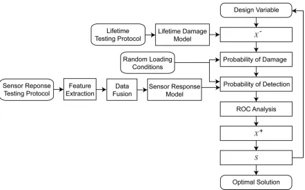
This dissertation presents a sensor optimization method for a network of embedded sensors applied for structural health monitoring of an airframe or airframe component. A flowchart of
the optimization process is shown in Figure 1.1. The method is applied to the specific case of a laminated composite plate with embedded fiber Bragg grating sensors subjected to low velocity impacts. This particular example highlights the differences in sensor placement
strategies between surface mounted and embedded sensors. Chapter 2 outlines the problem statement and the random loading cases that will be used to perform the sensor placement
optimization. Chapter 3 describes the experimental testing protocol to quantify the lifetime of the laminate as a function of quantity of embedded sensors, including the variability due to the specimen fabrication and the damage initiation and propagation. The results of these
experiments are collected to form a lifetime damage model as a function of the optical fiber spacing. Chapter 4 describes the performance of four damage measures for FBG reflected
spectra: spectral bandwidth, cross-correlation, number of peaks and fractal dimension. This chapter identifies which damage measure yields the most reliable indicator of damage in a complex, realistic strain environment. Chapter 5 presents a second experimental testing
protocol, this time to quantify the sensor response as a function of the laminate remaining lifetime and sensor locations. The resulting sensor response model is established including a
7
receiving operating characteristic analysis and then combined with the lifetime damage model to generate an optimal sensor placement solution. Results of this optimization for
different sensor feature extraction methods are presented in Chapter 6. Finally, Chapter 7 discusses the conclusions drawn from this research and recommends future research
8
9
CHAPTER 2
PROBLEM STATEMENT
For the embedded sensor placement optimization problem we define the lifetime benefit function, S, to be maximized, as
S X X (2.1) where X represents the negative effects of the embedded sensor on the structural lifetime and X represents the positive effects of the condition based monitoring enabled by the sensor information. Therefore, a net lifetime benefit to applying embedded FBG sensors
exists when SS0 with S0 X X0 0 and a net loss exists when SS0. The two functions
X and X should be scaled appropriately such that their relative weights are appropriate for a given application. We will calculate each of these functions empirically based on experimental data.
In order to demonstrate the application of the embedded sensor placement
optimization method of Figure 1.1, we will apply it to a particular problem. In order to highlight the optimization process itself, we have chosen a simple structural component, a
10
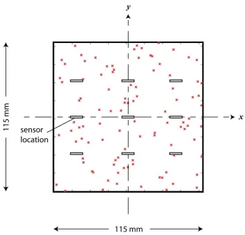
methodology to more complex structural geometries will be discussed in the concluding remarks. We will optimize embedded sensor placement in a 115 mm x 115 mm laminated
plate, constructed from 24 layers of 2 x 2 twill woven graphite fiber–epoxy pre-preg, with a total thickness of 4 mm (see Figure 2.1). This particular geometry and material system was
chosen such that previous experimental data could be used to quantify the impact response and lifetime of the component (Park et al., 2010).
The design variable for this optimization example is the optical fiber spacing, . As mentioned earlier, this spacing is based on is based on the method optical fibers are
embedded between laminae. Here we consider that optical fibers are only embedded at the laminate midplane and are all aligned in the same direction to prevent local stress
concentrations when they intersect (Garrett et al., 2009). A range of = 0.087 to 1.422 optical fibers/cm was applied. The specific sensors used to identify the presence of damage in this example are fiber Bragg grating (FBG) sensors. For a given optical fiber spacing, the
number of optical fibers across the length of the specimen was calculated and locations identified, symmetrically placed about the center of the specimen. Optical fibers located within 8 mm of the outer edges were not included, since these have been previously shown to
cause a rapid increase in the growth of delamination from the outer edges of the laminate. The same restrictions were applied to the previous experimental studies (Park et al., 2010).
11
sensors per fiber does not decrease the lifetime of the laminate, it does increase the data acquisition requirements. Since the laminate is quasi-isotropic and the boundary conditions
symmetric, there is not an increased information benefit to having a higher spacing of sensors in one direction over the other, therefore the sensor distribution in the x and y directions was
chosen to be the same. Figure 2.1 shows the FBG sensor distribution for the case where three optical fibers are embedded in the laminate.
One hundred impact loading cases were generated to calculate the probabilities of
damage and detection of this damage by the sensor network. The applied impact loading, F,
was represented as a function of random variables including both the magnitude and location of the impact,
2 0 0 0, 0
1 , ,
2
i i
F v x y mv x y (2.2)
where is the Dirac delta function, m and vi are the mass and velocity of the impacting
object respectively, and x0 and y0 are the location of the impact. The variables x0 and y0
were assumed to be uniformly distributed throughout the in-plane laminate dimensions,
0 0
57.5 mm x 57.5 mm, 57.5 mm y 57.5 mm
.
The
x y0, 0
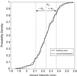
location of each of the one hundred generated loading cases is shown in Figure2.2. The mass of the impactor was assumed to be m = 5.5 kg and the impact velocity was
assumed to have a normal distribution with a mean velocity m = 2.23 m/s and a standard
deviation D= 0.11 m/s to correlate with previous experimental data (Park et al., 2010). The
12
that of the one hundred generated impact velocities are shown in Figure 2.2. For real
13
14
15
CHAPTER 3
LIFETIME DEGRADATION
3.1 BACKGROUND
Fiber-reinforced polymer composites have become widely used as replacements for traditional metallic materials in aerospace applications. Their use has resulted in lightweight,
high performance airframe skins, stiffeners, and structural joints. As the failure mechanisms of these laminated structural components are significantly different than those of
homogenous materials, new in situ damage assessment methods must be implemented to assure the reliability of these components. Internal damage in the form of interrelated delaminations, fiber breakage, and matrix cracking can rapidly lead to catastrophic failures.
One of the most promising techniques to assess internal damage in these composite laminates is the embedment of an array of sensors directly into the composites (Garrett et al., 2009).
The authors have previously demonstrated that in situ assessment of a woven composite laminate through embedded fiber Bragg grating (FBG) sensors can accurately be used to identify the presence and form of damage modes prior to catastrophic failure (Garrett et al.,
16
of the sensors within the interior of the laminate, that is, closer to the location of the failure modes.
In general, the more sensors that are available within a given structural volume, the higher the fidelity of the damage state reconstruction and therefore the more accurate the
remaining lifetime prediction for a given structural component. However, this increased fidelity is not without additional costs. When designing a surface mounted sensor network, increasing the number of sensors increases the hardware costs, installation costs and data
collection requirements of the system. While the same is true for embedded sensors, a more critical penalty is the potential negative impact of the network presence on the material
properties of the host material system. To properly design an embedded sensor network one must therefore be able to accurately quantify this penalty for a given structural system.
While the specific role of the embedded sensor-host interaction on the performance
and lifetime of a structural component depends upon the particular loading conditions and properties of the host material system, some general conclusions can be drawn from previous
experimental studies. Most of these previous efforts have focused on the in-plane properties of laminates with embedded optical fibers. Jensen and Pascual (1990) and Jensen et al. (1992) concluded that large quantities of embedded optical fibers degraded the tensile and
compressive behavior of graphite/bismaleimide laminates. The magnitude of the tensile strength, stiffness, and compressive strength reductions were linearly proportional to the
17
maximum measured effect on compressive strength was on the order of 30%. The presence of the embedded optical fibers also had a larger effect on the compressive strength than on
the compressive stiffness of composite laminates, meaning that it is the lifetime rather than the performance of a laminate that is critically affected by the presence of the optical fibers.
The orientation of the embedded optical fibers relative to the host material geometry also affects the sensor-host interaction. Jensen and Pascual (1990) and Jensen et al. (1992) found that optical fibers embedded perpendicular to the adjacent graphite fibers induced the largest
reductions in the mechanical properties of composite laminates. Experimental studies have also been performed on the lifetime of laminates with embedded sensors subjected to
in-plane fatigue loading, with similar conclusions (Kuang and Cantwell, 2003).
Few, if any, investigations have evaluated the negative effects of embedded optical fiber sensors on laminates subjected to low velocity impact loading. The presence of optical
fibers could induce local variations in the interlaminar stress distributions, potentially leading to premature delaminations. There is thus a need to understand and quantify how the
embedded optical fiber influences both the initiation of damage and the propagation of critical damage which determines the remaining lifetime of the laminate. The only previous studies in the literature directly addressing the role of the embedded sensors during low
velocity impact loading are Sirkis et al. (1994) and Sirkis and Chang (1994). The authors embedded a single optical fiber at the midplane of graphite fiber-epoxy laminates with
18
of the specimens was performed to compare the induced delamination regions. The laminates were then sectioned to observe micro-cracking surrounding the optical fiber and in other
regions of the laminates. As expected, delamination was the dominant failure mode for all tested laminates. The testing demonstrated no visible effects on the formation of transverse and longitudinal cracks due to embedded optical fibers with diameters below 600 μm. In
some cases, the authors thought that the optical fibers had even acted as crack arrestors. Additionally, matrix cracks did not initiate in the resin rich zone surrounding the embedded
optical fibers. These results at the micro-level are consistent with the measured delamination areas, which were the same for specimens with and without the optical fibers. Therefore, the
embedded optical fibers of these diameters have no measurable influence on the initiation and growth of damage within the laminates. These results have been verified when sensors were included in the optical fibers in Chang and Sirkis (1997).
However, a significant barrier exists to extrapolate these observations of a single embedded optical fiber to a quantitative model of the role of embedded optical fiber spacing
on the damage initiation and propagation in laminates due to low-velocity impact loading. The extremely localized nature of failure initiation creates a large variability in the measured lifetime of identical specimens without embedded optical fibers. Furthermore, once
embedded sensors are added to the laminate, these localized failures are highly sensitive to the local material geometry surrounding the optical fiber and the optical fiber placement
19
In this investigation, we perform an experimental study of the global response of woven graphite fiber-epoxy laminates subjected to multiple low velocity impacts with
various spacing of embedded optical fibers. The goal is to quantify the role of optical fiber spacing on the degradation of global material properties of the host material system. A large
number of specimens were experimentally tested to measure the changes in the statistical distributions of the maximum contact force and total dissipated energy of the laminates. These results are then interpolated to yield a model of these properties as a function of
embedded optical fiber spacing. The optical fibers in this chapter do not contain FBG sensors, as the presence of sensors does not affect the response of the host material system.
Previous studies have demonstrated the performance of FBG sensors following the same specimen fabrication and testing procedures used in this work (Garrett et al., 2009). While the resulting numerical values of the model would be different for another material system or
impact loading history, the goal of this chapter is to derive the testing protocol and data analysis method to apply to any laminate configuration.
3.2 EXPERIMENTAL METHODS
3.2.1 Specimen Fabrication
20
x 115 mm2 with a resulting thickness of 4 mm (Figure 3.1). All optical fibers were embedded at the midplane. All optical fibers had a polyimide coating, chosen to maximize the adhesion
between the optical fiber and the surrounding matrix. The polyimide also provides additional stiffness to the optical fiber and prevents transmitted power losses due to transverse
compressive residual stresses. Garrett et al. (2009) measured the response of FBG sensors embedded in composite laminates and demonstrated that the optical fibers had good adhesion and low loss levels when using the same fabrication procedures used in this study. A single
step technique was used to assemble the uncured prepreg laminate on each side of the optical fibers and cure the entire assembly (Park et al., 2009). A layer of Mylar release film and
peel-ply were first placed on a surface. The first 12 layers of prepreg were placed on an aluminum plate on the peel-ply and the optical fibers were placed on top at 0° relative to the orientation to the carbon fabric and parallel to each side of the sample. To maintain the tension in the
optical fibers and the correct fiber spacing, the ends of the fibers were taped to a grooved frame surrounding the plate as shown in Figure 3.2. The remaining 12 layers of prepreg were
then assembled on top of the fibers. To protect the fibers from excess amount of the epoxy resin during the curing cycles, additional plumbers’ putty was placed around the fibers on
each side of the sample. This additional putty did not affect transmission through the optical
fibers in previous experiments (Garrett et al., 2009). A layer of peel-ply and Mylar release film were then added to the top of the sample. The release film was sealed with plumber’s
21
stepped temperature profile up to 80°C and a constant pressure of 458 kPa. An additional 30 minutes of pressure was applied during cooling of the laminate. This procedure produced
highly reliable bonding of the laminate and low void concentrations. The edges of the laminate were not trimmed as they were outside the area to be clamped and did not affect the
impact response.
A total of 80 specimens were fabricated, divided into four sets, depending on the optical fiber spacing (Figure 3.1):
1) 20 specimens with no embedded optical fibers (Specimens N1 - N20);
2) 20 specimens with 5 optical fibers at a spacing of 24.6 mm (0.406 optical fibers/cm)
referred to as low spacing specimens (Specimens LD1 - LD20);
3) 20 specimens with 10 optical fibers at a spacing of 10.9 mm (0.914 optical fibers/cm)
referred to as medium spacing specimens (Specimens MD1 - MD20);
4) 20 specimens with 60 optical fibers at a spacing of 1.7 mm (5.994 optical fibers/cm)
referred to as high spacing specimens (Specimens HD1 - HD20).
3.2.2 Low Velocity Impact Experiments
Composite materials sustain the damage in the interior of the laminate that is not detectable during visual inspection. Low velocity impacts are therefore prone to cause this type of
22
transfer to locations away from the point of impact. Since the contact time between the projectile and the composite is considerably higher, the impact loading induces a localized
response with global deformation.
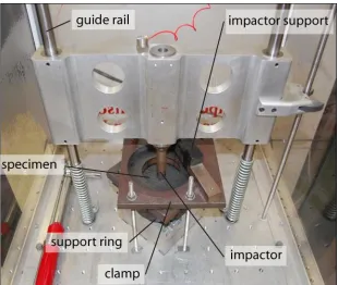
All specimens were mounted in a drop tower and subjected to multiple low velocity
impacts until failure. The instrumented impact drop tower, shown in Figure 3.3, consists of a 19 mm diameter hemispherical hardened steel impactor fixed to an aluminum crosshead. The entire crosshead assembly has a mass of 5.5 kg. The composite laminates were securely
clamped by a 76.2 mm inner- and 152 mm outer diameter circular steel ring, sandwiched by a neoprene mat to distribute pressure evenly over the boundary. The impactor contacted the
specimen surface at a nominal velocity of 2.3 m/s, providing an impact energy of 14.5 J. The rebound of the crosshead was manually arrested to prevent rebound impacts during a single strike event. Failure of the specimen was considered to be when the impactor perforated the
specimen. Throughout each impact event, the acceleration of the impactor was collected from a piezoelectric accelerometer mounted on the crosshead and the position of the impactor was
obtained from a non-contacting magnetorestrictive sensor on the guide rail. Both sensors were interrogated with an oscilloscope at 50 kHz, triggered by the position sensor at a fixed distance above the specimen surface height. This height measurement was recorded after
each strike by resting the crosshead on the specimen surface. The impactor contact force profile was determined from the accelerometer, and filtered using a 0.46 ms moving average.
23
The energy dissipated by the specimen during each strike, ED, was calculated from
the velocity data through Equation (3.1),
2 2
1 2
D i o
E m v v (3.1)
where m is the mass of the impactor, vi the velocity of the impactor just prior to contact with
the specimen and vo is the exit velocity of the impactor just after contact with the specimen.
The energy dissipation due to friction between the crosshead and the guide rails was
negligible. The total amount of energy dissipated over all strikes until failure of the specimen was also determined for each specimen. The energy dissipated by the specimen during impact was chosen as the measured of laminate lifetime since it did include the elastic
response of the laminate, only the energy which was assumed to be due to damage accumulation with the laminate. A threshold level of impact energy was assumed to exist,
24 3.3 RESULTS
3.3.1 Input Velocity
All four sets of specimens described above were subjected to multiple low velocity impacts until complete perforation of the specimen. Before we considered the response of each set of specimens, we first verified that the statistical distribution of the input loading conditions was
the same for all four sets. Since the crosshead was manually released for each specimen, some variation in the input velocity is expected. Figure 3.4(a) plots a histogram of the input
velocity data, calculated from the position sensor. Data are plotted for the total of 1856 strikes that were applied to the 80 specimens tested. The mean value and standard deviation of the input velocity were 2.254 m/s and 0.109 m/s, respectively. A best fit normal
distribution to the input velocity data is also plotted in Figure 3.4(a). Due to the large number of samples collected, the histogram is a smooth representation of the data. However, to
confirm that the assumed Gaussian distribution of Figure 3.4(a) is an appropriate distribution, Figure 3.4(b) shows the calculated cumulative distribution of the experimental data superimposed on the assumed normal distribution of Figure 3.4(a). The normal distribution
curve cannot be seen in Figure 3.4(a) as it follows the experimental data closely. The standard deviation of the input velocity data was also reasonably low at less than 5% of the
25
The mean input velocity and standard deviation was also compared with each of the four specimen sets tested, as plotted in Figure 3.4(c). The goal of this calculation was to
verify the consistency of the input velocities between the specimen sets. The difference in mean input velocity between each set was within one standard deviation, indicating that the
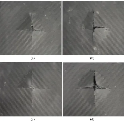
input loading conditions were statistically equivalent between all sets. The rear view (opposite to the impacted surface) of four representative specimens after final perforation is shown in Figure 3.5. The final failure mode of all specimens was extremely similar and
symmetric due to the isotropic nature of the particular two-dimensional twill woven composite used. As the input conditions and resulting failure modes were the same for each
embedded optical fiber spacing, it is appropriate to use the same damage measures to compare their performance.
3.3.2 Total Dissipated Energy
Twenty specimens (N1– N20) were fabricated without embedded optical fibers to establish a benchmark for the impact response of the laminate material system. For each specimen, the number of strikes to failure, the average initial velocity per strike, the maximum contact force
per strike summed over the laminate lifetime (total maximum contact force), and the total energy dissipated by the laminate over its lifetime were determined. The results for
26
therefore be used to compare with the other samples fabricated with different spacing of embedded optical fibers.
As for the data of Figure 3.4, we plot the cumulative distribution of the data in Figure 3.6 and compare it to the theoretical cumulative distribution of the best fit normal
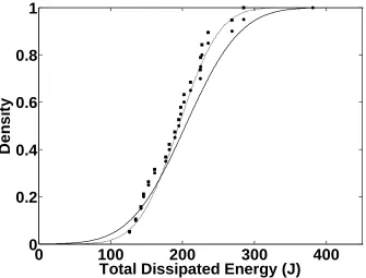
distribution. In contrast to the input velocity data, there are only 20 data points from which to calculate the distribution, therefore the cumulative distribution does not fit as well to the experimental data. We observe that two specimens had unusually large values of total
dissipated energy, above 390 J. These two specimens (Table 3.1) survived an unusually high number of strikes before failure, 48 and 49, increasing the total calculated dissipated energy.
Previous testing had demonstrated that when significant delamination occurs rapidly in the specimen, the specimen was held together by the clamped boundary conditions; however the delaminated surface moved freely during impact. The impactor did not necessarily penetrate
the specimen although the specimen had failed and the total dissipated energy was artificially inflated for the specimen (Pearson et al., 2007). Assuming this to be the case for specimens
N5 and N14, these were identified as outliers and the cumulative distribution was plotted without these data points in Figure 3.6. For this revised data set, the best fit normal distribution closely matched the experimental data. Collecting more data points would
improve the cumulative distribution plot of the experimental data; however Figure 3.6 indicates that the calculated normal distribution (without outliers) is a reasonable fit to the
27
standard deviation of total dissipated energy for specimens N1-N20 were 199.7 J and 46.7 J, respectively.
Specimens LD1-LD20 each had five embedded optical fibers at a spacing of 0.406 fibers per cm. The specimens LD1-LD20 were subjected to multiple low velocity impacts
following the same procedure as for the earlier reference specimens. The results for specimens LD1-LD20 are reported in Table 3.2. Once again the normal distribution assumption was validated for the data by plotting the cumulative distribution in Figure 3.7.
For this data set one specimen, LD 4, survived 48 strikes, resulting in an unusually high total dissipated energy of 381 J. This specimen was considered an outlier and the cumulative
distribution was recalculated without this specimen (Figure 3.7). The resulting cumulative distribution matched the measured data set well. From this distribution, the mean value of the total dissipated energy was calculated to be 5.9 J lower than that of the reference specimens
N1-N20. This was a decrease of 3.0%.
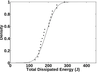
Specimens MD1-MD20 contained embedded optical fibers at a spacing of 0.914
fibers per cm, twice that of the low spacing specimens. The results for specimens MD1-MD20 are reported in Table 3.3. The normal distribution assumption was validated for the data by plotting the cumulative distribution in Figure 3.8. No outliers were found in this data
set. The mean value of the total dissipated energy further decreased and was 10.0 J lower than that of the reference specimens N1-N20, a decrease of 5.0%.
28
be practical for any realistic application, it was chosen as an extreme value of sensor spacing to better understand the relationship of laminate lifetime to the embedded optical fiber
spacing. The results for specimens HD1-HD20 are reported in Table 3.4. The normal distribution assumption was validated for the data by plotting the cumulative distribution in
Figure 3.9. The mean value of the total dissipated energy was 10.2 J lower than that of the reference specimens. This decrease in total dissipated energy was not statistically significant from that of the medium spacing specimens.
3.3.3 Total Maximum Contact Force
While the total dissipated energy can be viewed as a measure of the laminate lifetime, the total maximum contact force is related to the laminate stiffness, therefore we present contact
force results in this section. The maximum contact force per strike was calculated from the filtered impactor acceleration data and then summed over the lifetime of the laminate. The
results for all specimens are reported in the Appendix. In Figure 3.10, we plot the cumulative distribution of the total maximum contact forces for each specimen set and compare them to the theoretical cumulative distribution of the best fit normal distribution. For the reference
and low spacing specimens, the cumulative distribution is plotted both with and without the outliers (those specified in section 3.3.2) removed. As for the case of the total dissipated
29
in Figure 3.10. Additionally, with the exception of the low spacing specimens, the mean value of the data decreased with increasing spacing of optical fibers, ranging from 125.9 kN
for the reference specimens to 101.6 kN for the high spacing specimens.
3.4 DISCUSSION
Figure 3.11 summarizes the total dissipated energy and total maximum contact force data
obtained from the various specimen sets. These results are also plotted in Figure 3.12(a) and (b) as a function of optical fiber spacing. Both parameters decreased rapidly for low optical
fiber spacing and quickly reached a threshold value at approximately 1.0 optical fibers/cm. The standard deviation of the dissipated energy also decreased with optical fiber spacing, but at a faster rate than the mean value. The standard deviation of the total maximum contact
force did not show a consistent behavior. While it is difficult to draw conclusions from only the four spacing fabricated, a fit to the dissipated energy and maximum contact force data
was performed to illustrate the data trends. Based on the form of the data, an exponentially decreasing function was chosen for both the mean and standard deviation. For the dissipated energy, ED, the fits are:
189.7J 10J exp 2.5 cm / fibers
D
E (mean)
38.7J 8.0J exp 1.5 cm / fibers
D
E (standard deviation) (3.2)
30
101.6kN 35kN exp 1.7 cm / fibers
F
C (mean)
23.0kN 9.0kN exp 0.6 cm / fibers
F
C (standard deviation) (3.3)
These data trend curves are also plotted in Figures 3.12(a) and (b). The average total
maximum contact force of the low spacing specimens was 131.5 kN, above that of the reference specimens. This result was not expected based on the physical problem; therefore an exponential decreasing function was still applied in Equation (3.3).
There was a significant amount of scatter in the lifetime of the laminate specimens, even with identical specimen fabrication and impact loading procedures. This scatter is due
to the localized nature of the failure modes and their high sensitivity to variations in the local microstructure. It was expected that the percent standard deviation of the total dissipated
energy would increase with embedded optical fiber spacing, as the introduction of the optical fibers adds uncertainty to the local microstructure. The fact that the percent standard deviation decreased with embedded optical fiber spacing indicates that above the threshold
spacing, the optical fibers at the midplane dominated the critical failure mode of the laminate. This change in failure mode reduced the variability in specimen lifetime due to the local
microstructure. In other words, above the fiber spacing threshold value, the fibers were within their mutual radius of influence and the failure mode was presumably controlled by the interaction of the residual stress concentrations in the matrix rich zones surrounding the
optical fibers. This is consistent with the existence of the threshold value of the total energy dissipated at failure. Specimens with additional embedded optical fiber spacing could be
31
The laminate stiffness, represented by the maximum total contact force, demonstrated the same behavior although the percent standard deviation was independent of optical fiber
spacing. Specimen stiffness is not strongly influenced by perturbations to the local microstructure; therefore the standard deviation was not expected to be influenced by the
embedded optical fiber spacing. In these tests, the specimen stiffness decreased by a maximum of 19.3% percent due to the presence of the optical fibers.
3.5 CONCLUSIONS
In this chapter, we experimentally measured the impact resistance of laminated woven carbon fiber-epoxy specimens with different spacing of optical fibers embedded at the laminate midplane. Even for identical material systems and fabrication processes, there was a
high variation in the number of strikes to failure, maximum contact force and total dissipated energy between specimens. Analysis of the input loading conditions for the different
specimen sets demonstrated that the input velocity distributions were normal distributions and identical between the various sets of specimens. The final failure modes were also consistent between specimen sets with different embedded optical fiber spacing. At low
optical fiber spacing, the total energy dissipated by the specimen and the total maximum contact force over the lifetime of the specimen decreased rapidly with increasing optical fiber
32
failure mode of the laminate and the laminate lifetime and stiffness were not sensitive to embedded optical fiber spacing.
The role of the embedded optical fibers is highly dependent upon a multitude of parameters including local host material geometry and properties, embedment locations,
impact loading history (location and energy level) and component geometry. The contribution of this chapter is thus a methodology to collect and analyze quantitative data on the impact of the sensor presence on the stiffness and lifetime of laminated structures. This
methodology could be applied for any host material system and loading history in order to optimize the spacing and location of embedded optical fiber sensor networks for future smart
33
34
35
36
Figure 3.4 Initial velocity data from all 80 samples: (a) histogram of data and (b) cumulative distribution plot. Best fit to normal distribution is also plotted in (a) as solid line and cumulative distribution calculated from this normal distribution plotted in (b) as solid line. (c) Plot of average initial velocity between various sets of optical fiber spacing. Error bars
37 (a)
39
(a) (b)
(c) (d)
40
0
100
200
300
400
0
0.2
0.4
0.6
0.8
1
Total Dissipated Energy (J)
D
e
n
s
ity
Figure 3.6 Total dissipated energy data from 20 samples without embedded optical fibers (N1-N20): Cumulative distribution. Experimental data plotted with (circles) and without (squares) outliers. Best fit to normal cumulative distribution without outliers is plotted with
41
0
100
200
300
400
0
0.2
0.4
0.6
0.8
1
Total Dissipated Energy (J)
D
e
n
s
ity
Figure 3.7 Total dissipated energy data from 20 samples with low spacing of embedded optical fibers (LD1-LD20): Cumulative distribution. Experimental data plotted with (circles)
42
0
100
200
300
400
0
0.2
0.4
0.6
0.8
1
Total Dissipated Energy (J)
D
e
n
s
ity
Figure 3.8 Total dissipated energy data from 20 samples with medium spacing of embedded optical fibers (MD1-MD20): Cumulative distribution. Best fit to normal cumulative
43
0
100
200
300
400
0
0.2
0.4
0.6
0.8
1
Total Dissipated Energy (J)
D
e
n
s
ity
Figure 3.9 Total dissipated energy data from 20 samples with high spacing of embedded optical fibers (HD1-HD20): Cumulative distribution. Best fit to normal cumulative
44
Figure 3.10 Cumulative distribution of total maximum contact force for samples: (a) without embedded optical fibers (N1-N20); (b) with low spacing of embedded optical fibers (LD1-LD20); (c) with medium spacing of embedded optical fibers (MD1-MD20) and (d) with high
spacing of embedded optical fibers (HD1-HD20). Experimental data plotted with (circles) and without (squares) outliers. Best fit to normal cumulative distribution without outliers is
45
0
50
100
150
200
250
300
0
0.2
0.4
0.6
0.8
1
Total Maximum Contact Force (kN)
D
e
n
s
ity
(a)0
50
100
150
200
250
300
0
0.2
0.4
0.6
0.8
1
Total Maximum Contact Force (kN)
46
0
50
100
150
200
250
300
0
0.2
0.4
0.6
0.8
1
Total Maximum Contact Force (kN)
D
e
n
s
ity
(c)0
50
100
150
200
250
300
0
0.2
0.4
0.6
0.8
1
Total Maximum Contact Force (kN)
47
48 (a)
(b)
Figure 3.12 Plot of experimentally obtained (a) total dissipated energy and (b) maximum contact force. Mean values are plotted as circles and + one standard deviation plotted as
49
Table 3.1 Data from samples without embedded optical fibers. Specimen Number of
strikes to failure
Average initial velocity (m/s)
Total maximum contact force (kN)
Total dissipated energy (J)
N1 24 2.263 133.3 198.0
N2 22 2.259 116.8 183.7
N3 24 2.288 126.4 219.9
N4 24 2.289 130.6 207.7
N5 48 2.285 226.1 406.1
N6 16 2.277 86.3 147.5
N7 23 2.303 122.9 208.0
N8* 29 2.281 146.6 248.4
N9 30 2.277 162.8 238.1
N10 33 2.270 174.2 258.8
N11* 21 2.267 124.5 170.1
N12 21 2.273 109.8 188.2
N13 31 2.281 155.7 266.5
N14 49 2.287 251.1 391.3
N15 17 2.285 93.2 144.6
N16 23 2.267 119.4 191.7
N17 14 2.295 77.9 126.3
N18 16 2.275 84.5 142.7
N19 20 2.254 108.3 166.1
N20 37 2.285 192.4 288.0
*For specimen N8, acceleration and position data were not collected for strike 21. For specimen N11,
50 Table 3.2 Data from samples with low spacing fibers.
Specimen Number of strikes to failure
Average initial velocity (m/s)
Total maximum contact force (kN)
Total dissipated energy (J)
LD1 35 2.246 185.4 268.9
LD2 22 2.251 114.4 176.5
LD3 19 2.249 108.0 142.3
LD4 48 2.244 231.6 381.3
LD5 23 2.251 130.5 181.7
LD6 20 2.195 110.6 152.5
LD7 28 2.269 152.9 235.5
LD8 30 2.230 160.7 225.2
LD9 24 2.239 119.3 211.0
LD10 26 2.238 143.5 194.7
LD11 26 2.235 147.1 197.6
LD12 30 2.220 162.6 227.3
LD13 17 2.231 93.4 135.1
LD14 24 2.268 126.6 201.9
LD15 28 2.262 155.9 224.9
LD16 15 2.255 84.5 126.3
LD17 19 2.253 101.1 161.1
LD18 23 2.256 123.6 189.2
LD19 36 2.244 185.1 285.0
51
Table 3.3 Data from samples with medium spacing fibers. Specimen Number of
strikes to failure
Average initial velocity (m/s)
Total maximum contact force (kN)
Total dissipated energy (J)
MD1 36 2.276 183.9 284.3
MD2† 21 2.266 103.8 177.3
MD3 16 2.268 82.1 144.6
MD4† 18 2.292 98.6 159.5
MD5 30 2.278 164.3 243.6
MD6 20 2.261 110.5 161.9
MD7† 22 2.262 120.4 180.6
MD8 25 2.251 111.5 244.5
MD9 19 2.233 98.3 167.6
MD10 16 2.257 78.7 150.7
MD11 19 2.227 89.5 174.9
MD12 22 2.263 105.4 202.1
MD13 24 2.251 114.6 221.0
MD14† 21 2.262 101.7 203.6
MD15 17 2.258 89.4 150.0
MD16 22 2.245 102.1 208.6
MD17 24 2.242 124.5 213.1
MD18 17 2.245 82.4 157.7
MD19 14 2.238 69.2 129.8
MD20 23 2.241 105.7 218.8
†For specimen MD2, acceleration and position data were not collected for strike 11. For specimen MD4,
52 Table 3.4 Data from samples with high spacing fibers.
Specimen Number of strikes to failure
Average initial velocity (m/s)
Total maximum contact force (kN)
Total dissipated energy (J)
HD1 10 2.212 44.5 97.9
HD2 14 2.243 65.4 135.7
HD3 24 2.232 114.1 226.1
HD4 18 2.177 81.4 140.8
HD5 23 2.255 121.0 211.9
HD6 25 2.214 126.0 219.9
HD7 19 2.226 95.6 173.3
HD8 18 2.219 86.3 161.5
HD9§ 21 2.348 112.9 230.8
HD10 19 2.250 96.5 210.6
HD11 17 2.312 82.2 192.7
HD12§ 24 2.202 116.1 234.4
HD13 20 2.182 99.7 171.6
HD14 25 2.202 138.8 200.6
HD15 25 2.278 128.2 247.0
HD16 21 2.268 95.2 228.3
HD17 20 2.193 99.2 184.2
HD18 17 2.216 88.3 151.0
HD19 22 2.185 117.7 185.2
HD20 24 2.204 123.6 185.8
§For specimen HD9, acceleration and position data were not collected for strike 5 and 10. For specimen HD12,
53
CHAPTER 4
DAMAGE MEASURES
4.1 BACKGROUND
The optical fiber Bragg grating (FBG) sensor has been commonly applied as a strain sensor for many applications. Typically the Bragg wavelength peak shift is converted into a measure
of the strain component along the axis of the optical fiber. However, when applied near regions of strain concentrations or damage in a material, the reflected FBG spectrum often
shows significant distortion (Peters et al., 2001; Park et al., 2010; Epaarachchi et al., 2010). This distortion is due to strain gradients, multiple strain components or non-uniformities or discontinuities in the strain field along the FBG axis and is theoretically predictable.
Extracting information on these strain states from the measured FBG reflected spectrum is therefore potentially useful for structural health monitoring.
When a detailed analysis is required, the distorted FBG reflected spectrum can be fit to known strain states (Huang et al., 1995; Minakuchi et al., 2007), or an inverse optimization algorithm applied to invert the applied strain field from the spectrum (Gill et al., 2004).