Performance Enhancement by Exploiting the Spatial Domain for Cost, Space and Spectrum Constraint 5G Communication

(1)

Scholarship@Western

Electronic Thesis and Dissertation Repository

4-30-2018 1:00 PM

Performance Enhancement by Exploiting the Spatial Domain for

Cost, Space and Spectrum Constraint 5G Communication

Golara Zafari

The University of Western Ontario Supervisor

Wang, Xianbin

The University of Western Ontario

Graduate Program in Electrical and Computer Engineering

A thesis submitted in partial fulfillment of the requirements for the degree in Master of Science © Golara Zafari 2018

Follow this and additional works at: https://ir.lib.uwo.ca/etd

Part of the Systems and Communications Commons

Recommended Citation Recommended Citation

Zafari, Golara, "Performance Enhancement by Exploiting the Spatial Domain for Cost, Space and Spectrum Constraint 5G Communication" (2018). Electronic Thesis and Dissertation Repository. 5400.

https://ir.lib.uwo.ca/etd/5400

This Dissertation/Thesis is brought to you for free and open access by Scholarship@Western. It has been accepted for inclusion in Electronic Thesis and Dissertation Repository by an authorized administrator of

(2)

With everlasting increase of connectivity demand and high speed data communication, lots

of progresses have been made to provide a sufficient quality of services (QoS). Several

ad-vanced technologies have been the cornerstone of this trend in academia as well as in industry.

Nevertheless, there are some implementation challenges, which needs to be closely

investi-gated. In this thesis, among all challenges, we elaborate on those related to number of radio

frequency (RF) chains and resource scarcity.

The principle idea behind our proposed initial solution is to exploit the spatial domain as an

additional degree of freedom. To be more specific, we benefit from spatial domain and antenna

index in a multiple-input multiple-output (MIMO) system with dual-polarized (DP) antennas

to convey the information. We develop a two-stage algorithm to groups the antennas which

ends up to the optimum performance. Another advantage of this proposed algorithm is the

complete complexity reduction of exhaustive search over the whole available space.

Moreover, due to the continuous growth of demands which results in spectrum scarcity, we

investigate the extension of long term evolution (LTE) spectrum. Such a paradigm shift is

real-ized to offload part of the data to unlicensed band, which has been initially dedicated to other

standardizations such as wireless local area networks (WLAN). As both LTE and wireless

fi-delity (Wi-Fi) networks have been widely deployed with solid infrastructures, it is significantly

important to make their coexistence viable with a cost-effective approach which inherently

re-quires the minimum protocol modification. Thus, we take the advantage of spatially located

multiple antennas of base station (BS) and access point (AP) for the sake of beamforming and

interference reduction.

In addition to network coexistence, we approach the resource scarcity from the non-orthogonal

multiple access (NOMA) point of view, where users share the frequency and time resources

and are differentiated in power domain. In particular, we closely consider those users with

limited number of RF chains. Similar to our first approach, we utilize spatial modulation (SM)

in user end and after evaluating their performance, we propose to consider the capacity of SM

NOMA to elaborate the impact of pairing on the achievable sum rate performance.

Keywords: MIMO, SM, NOMA, antenna selection

(3)

This thesis has been written by Golara Zafari under supervision of Dr. Xianbin Wang. The

ma-terial presented in Chapter three and four have been published in IEEE Vehicular Technology

Conference as follows

G. Zafari, M. Koca, X. Wang and M. G. S. Sriyananda, “Antenna Grouping in

Dual-Polarized Generalized Spatial Modulation,” 2017 IEEE 86th Vehicular Technology Conference

(VTC-Fall), Toronto, ON, 2017, pp. 1-6.

G. Zafari and X. Wang, “Cognitive Co-Existence of Unlicensed Wireless Networks through

Beamforming,” 2017 IEEE 86th Vehicular Technology Conference (VTC-Fall), Toronto, ON,

2017, pp. 1-5.

(4)

First, I would like to express my sincere appreciation to my supervisor Dr. Xianbin Wang for

his guidance and support. I would like to express my gratitude to Dr. Wang for providing me

with the opportunity to work under his supervision. It was under his guidance and support that

I was able to accomplish the program. I would also like to thank the examining committee, Dr.

Shami, Dr. Badrkhani Ajaei, and Dr. Mao for their constructive suggestions on my research

and thesis.

Special thanks to Dr. Junghoon Suh, Dr. Edward Au, and Dr. Osama AboulMagd from

Huawei Corporation for their insightful hints and helpful discussions. My sincere appreciation

to Dr. Koca for all his encouragements and valuable suggestions.

Words cannot express how grateful I am to have my lovely family. I would like to thank my

parents for their endless love, support, and advice that always enlighten my way. Many thanks

to my dear brother Zafar and his wife Elahe for making me so determined to achieve all my

goals. I miss you all. I also feel so much fortunate to have my beloved husband, Behzad. His

stubborn integrity, his knowledge, and his stickler of perfection were a true inspiration for me

to accomplish this program.

Last but not least, I would like to thank all dear friends in our research team. Specially,

Hessam, Sabin, Hao, Monica, Yanan, and Shery for all time we spend together

(5)

Abstract ii

Co-Authorship Statement iii

Acknowlegements iv

List of Figures viii

List of Tables x

List of Abbreviations, Symbols, and Nomenclature xi

1 Introduction 1

1.1 Overview of Promising Communication Technologies . . . 1

1.2 Thesis Motivation . . . 2

1.3 Thesis Objectives . . . 3

1.4 Technical Contributions of the Thesis . . . 4

1.5 Scope of Thesis . . . 4

2 Principle and Detection Analysis of Spatial Modulation 6 2.1 Modulation in Space Domain . . . 6

2.1.1 Spatial Modulation Technique . . . 7

2.1.2 Multi-stream Generalized Spatial Modulation . . . 10

2.2 Detection Algorithms . . . 12

2.2.1 Low-complex Suboptimal Linear Detection . . . 12

Zero Forcing (ZF) Detection Algorithm . . . 12

Minimum Mean Square Error (MMSE) Detection Algorithm . . . 13

(6)

2.2.3 Optimal Maximum Likelihood Detection . . . 13

2.2.4 Log-Likelihood Detection Algorithm . . . 15

2.2.5 Performance Analysis of SM with Different Detection Algorithms . . . 19

3 Antenna Selection in Dual-Polarized Generalized Spatial Modulation 23 3.1 Introduction . . . 23

3.2 System Model . . . 25

3.2.1 TITO Scenario . . . 26

3.2.2 MIMO Scenario . . . 27

3.3 Proposed Antenna Grouping . . . 29

3.3.1 Selection of Group Indicators . . . 29

3.3.2 Selection of Inner Group Antennas . . . 30

3.3.3 Feasibility of the Algorithm . . . 30

3.4 Performance Analysis . . . 32

3.5 Simulation Results . . . 33

3.6 Conclusion . . . 35

4 Co-existence of LTE and Wi-Fi in Unlicensed Band 38 4.1 Introduction . . . 38

4.3 Wi-Fi Received Power Minimization . . . 42

4.4 UE Received SNR Maximization . . . 44

4.5 Simulation Results . . . 45

4.6 Conclusion . . . 49

4.7 Proof of Proposition 4.3.1 . . . 50

5 NOMA-based Communication with Spatial Modulation 52 5.1 Introduction . . . 52

5.3 Average Bit Error Rate Analysis . . . 55

(7)

5.4.1 User pairing in SISO NOMA . . . 60

5.4.2 User pairing in MIMO Scenario . . . 69

5.5 Capacity of SM-NOMA . . . 70

5.5.1 Simulation Results . . . 74

6 Conclusion and Future Work 76

Bibliography 77

Curriculum Vitae 84

(8)

2.1 Illustration of SM transmission algorithm [1]. . . 8

2.2 Successive interference cancellation approach [2]. . . 14

2.3 Block diagram of SM transmission and ML detection structure [3]. . . 15

2.4 Convolutional encoder with coding rate of 1/2 [4]. . . 18

2.5 Performance analysis based on LLR detection. . . 18

2.6 Comparison of spatial multiplexing and spatial modulation, 6 bits/subcarrier. . . 20

2.7 Comparison of spatial multiplexing and spatial modulation, 10 bits/subcarrier. . 20

2.8 Comparison of MRC and ML detection of SM. . . 21

2.9 2×2 SM-MIMO and SMX comparison based on LLR detection,R= 4. . . 22

2.10 4×4 SM-MIMO and SMX comparison based on LLR detection,R= 4. . . 22

3.1 DP antenna configuration with different number of antennas, a) Nt = 8 DP antennas, b)Nt =4 DP antennas. . . 29

3.2 An example of antenna grouping considering their distance and polarizations, assumingNt =32 DP antennas,m= 3, andNa= 2. . . 31

3.3 Performance comparison of the proposed algorithm with the optimum achiev-able ABEP and UP-GSM with different spatial correlation coefficients when Na =2, for a)R=3 bpcu, b)R= 4 bpcu. . . 36

3.4 Performance comparison of the proposed algorithm with the optimum achiev-able ABEP and UP-GSM with different spatial correlation coefficients when Na =3, for a)R=3 bpcu, b)R= 4 bpcu. . . 37

4.1 Networks coexistence and undesired interference from LTE-U on Wi-Fi. . . 41

4.2 Minimum received power by Wi-Fi AP vs. QoS threshold for UE, αg = −10 dB andαh ={−20,−10,0}. . . 47

(9)

dB andαg ={−20,−10,0}. . . 48

4.4 Maximum received SNR by UE vs. power threshold for Wi-Fi AP,αg = −10

dB andαh ={−20,−10,0}. . . 49

4.5 Maximum received SNR by UE vs. power threshold for Wi-Fi AP,αh = −10

dB andαg ={−20,−10,0}. . . 50

5.1 Principal of NOMA communication with SIC detection [5]. . . 53

5.2 Performance analysis of two users with NOMA transmission and same spectral

efficiencies, i.e.,R=4. . . 58

5.3 Performance analysis of two users with NOMA transmission and different

spectral efficiencies and different number of antennas. . . 59

5.4 Capacity comparison of NOMA and OMA, SISO,a2

n =1/5 anda2m= 4/5,K = 0. 61

5.5 Capacity comparison of NOMA and OMA, SISO,a2n =1/5 anda2m= 4/5,K = 5. 61

5.6 Capacity comparison of NOMA and OMA, SISO, a2

n = 1/5 and a2m = 4/5,

S NR=20 dB. . . 62

5.7 Probability of OMA outperforming NOMA vs. 1/N0,K = 0. . . 68

5.8 Probability of OMA outperforming NOMA vs. 1/N0,K = 5. . . 68

5.9 User pairing based on sum rate capacity,α2

1 =1/5 andα

2

2 = 4/5, Nt = Nr= 4. . 74

5.10 Capacity comparison between SM-NOMA and SM-OMA, α2₁ = 1/5 andα2₂ =

4/5,Nt = Nr= 4. . . 75

(10)

2.1 SM scheme, Mapping input bits to corresponding constellation symbols and

antenna space. . . 9

2.2 G-SM scheme, Mapping input bits to corresponding constellation symbols and

antenna space,Nt = 4,Na =2,m= 2, QPSK. . . 11

2.3 Simulation parameters. . . 17

3.1 Size of the search space for different values ofNaandm. . . 31

(11)

ABER Average bit error rate

AP Access point

bpcu Bits per channel use

BS Base station

CSMA/CA Carrier sense multiple access with collision avoidance

DIFS Distributed inter-frame space

DoA Direction of arrival

DP Dual-polarized

ES Exhaustive search

ESM Enhanced spatial modulation

FDMA Frequency division multiple access

GSM Generalized spatial modulation

G-SSK Generalized space shift keying

IAI Inter antenna interference

i.i.d Independent and identically distributed

IoT Internet of things

ISM Industrial, Scientific and Medical

LAA License-assessed access

LBT Listen before talk

LLR Log-likelihood ratio

LOS Line of sight

LTE Long term evolution

MIMO Multiple-input multiple-output

ML Maximum likelihood

MMSE Minimum mean square error

MRC Maximum ratio combining

NLOS Non line of sight

NOMA Non-orthogonal multiple access

(12)

PDMA Pattern division multiple access

QoS Quality of services

QSM Quadrature spatial modulation

RF Radio frequency

SIC Successive interference cancellation

SM Spatial modulation

SMX Spatial multiplexing

SNR Signal to noise ratio

SSK Space shift keying

TDMA Time division multiple access

TITO Two-input two-output

UE User equipped

U-NII Unlicensed National Information Infrastructure

UP Uni-polarized

Wi-Fi Wireless fidelity

WLAN wireless local area networks

XPD Cross-polar discrimination

ZF Zero forcing

(13)

Introduction

1.1 Overview of Promising Communication Technologies

It has been known that communication industry is the main leading industry for future life.

According to statistics [6], the global spending of this industry is estimated to approach 1428.9

billion U.S. dollars in 2018 and it keeps increasing even more in future. Applications of such

an industry demand for wide rang of requirements from high speed video streaming and

aug-mented reality to low-data/power-limited internet of things (IoT) devices and health-care

ser-vices. Obviously, providing such a diverse quality of service (QoS) including high speed, low

data rate, enhanced reliability and coverage neither can be achieved with the current wireless

infrastructure, nor by redesigning a single entity in mobile communication systems. Instead, it

can be achieved solely based on combination of several advanced transmission technologies.

To address the high data rate-centric demands, novel technologies such as small-cell

com-munication, densification, massive multiple-input multiple-output (MIMO) comcom-munication,

and millimeter wave communication have become the roadmap for telecommunication

indus-try and new standardizations [7].

Nevertheless, there are some bottlenecks in aforementioned technologies that make their

deployment to be challenging. The main challenges arise as a results of space limitation, power

restrain, and spectrum scarcity.

(14)

1.2 Thesis Motivation

As mentioned in the previous section, limited space, available power, and spectrum scarcity are

the main limitations in communication systems. As an example, massive MIMO is realized by

placement of the large number of antennas (in order of hundreds). Nevertheless, positioning

of these antennas together with all their analog elements (such as phase shifters and power

amplifiers) is subject to violate the cost and power limitation. On the other hand, packed

an-tenna implementation creates spatial correlation and degrades the performance of transmission.

Therefore, it is necessary to design a new transmission strategy with reduced radio frequency

(RF) chain while providing a reasonable data rate.

Another problem that arises with large number of antennas is energy consumption. To be

specific, every antenna element is accompanied by a RF chain and thus, increasing number of

antennas requires more RF chains. Moreover, each RF chain contains power amplifier (PA).

Considering the fact that 70% of the total energy in a base station (BS) is consumed by PA and

dissipated as heat [8], novel hardware design is a vital factor from energy/power efficiency point

of view. The significant of new power efficient technology with limited number of RF chains

becomes even more critical for applications such as low-power wearable and IoT devices. For

these reasons, designing a new transmission approach with sufficient trade-offbetween number

of RF chains and data rate needs to receive close study.

Spectrum scarcity is another limiting factor of future densified networks. One approach

to deal with this problem is to share the spectrum, which can be realized in either licensed or

unlicensed band. Spectrum sharing in licensed band has been widely studied under the main

category of horizontal and vertical sharing [9]. In horizontal spectrum sharing, entities have

the same priority while in vertical sharing, the secondary user has lower priority in comparison

with the primary user. Seeking the additional spectrum has further led to idea of benefiting

unlicensed band and offloading part of the long term evolution (LTE) data to the underutilized

unlicensed spectrum. Considering the fact that 2.4 GHz Industrial, Scientific and Medical

(ISM) and 5 GHz Unlicensed National Information Infrastructure (U-NII) bands are utilized by

low-power wireless local area networks (WLAN) enabled devices, shifting LTE to unlicensed

(15)

Another approach to cope with the resource scarcity and support the high traffic demand is

to create an overlap in the resources assigned to different users. In the conventional multi-user

techniques, orthogonal resources (non-overlapping resources) are assigned to different users

and thus the interference has been eliminated. Evidently, the number of users that can be served

is limited to the amount of resources. To address this restriction, a new direction of study,

namely non-orthogonal multiple access (NOMA) has become of broad and current interest.

Thanks to non-orthogonality aspect of NOMA, the number of users can be enlarged regardless

of available resources. It is worth mentioning that the space and power constraints as explained

earlier are even more emphasized in user ends, which highlights the significance of new energy

efficient transmission scheme which can be applied to users under NOMA transmission.

1.3 Thesis Objectives

The main objective of this thesis is to study the aforementioned challenges and difficulties of

next generation of wireless communication systems and develop novel approaches to alleviate

these problems. To be more specific, we aim to

• Design and evaluate a compact implementation of MIMO systems and reduce the number

of RF chains. Implementation of such a compact and energy efficient system is vital in

many applications specificly in low-power devices such as wearable devices and IoT

applications.

• Develop a spatially and efficient strategy for the coexistence of wireless fidelity

(Wi-Fi) and LTE networks in unlicensed band which barely depends on modification in the

current network infrastructure and protocols. In particular, we consider the interference

reduction of one network on the other one to provide a cost-effective concurrent networks

environment.

• Improve the network capacity with NOMA and for limited-power users who have

con-straint on the number of RF chains. It is crucial to achieve a sufficient capacity with

(16)

capac-ity by assigning the overlapped resources to the users while preserving the requirement

of energy-efficient single RF chain.

1.4 Technical Contributions of the Thesis

The main contribution of the thesis is as follows:

• In Chapter 3 we propose a novel two-stage optimum antenna grouping scheme in

gen-eralized spatial modulation (GSM) with dual-polarized (DP) antennas. In the first stage

of the proposed scheme, we select antennas with their polarizations as group indicators

followed by the second stage, which determines the potential antennas and polarizations

that can be selected within each group. The proposed algorithm directly chooses the

activated antennas and therefore, completely eliminates the necessity of search over an

extensive space.

• In Chapter 4, we propose to use the space dimension and beamforming to facilitate the

effective coexistence and inter-network coordination. Two distinct approaches to

eval-uate the proposed coexistence mechanism, namely, Wi-Fi received power minimization

and LTE user signal to noise ratio (SNR) maximization, have been investigated. The

two proposed algorithms are simulated to show the potential and effective feasibility of

coexistence between Wi-Fi and LTE in unlicensed spectrum.

• Chapter 5 focuses on muli-user scenario. We consider the uplink transmission where

each user is constraint with single RF chain due to the space consideration. We

imple-ment the non-orthogonal multiple access to enhance the network capacity. Doing so, we

first, analyze the performance of SM-based uplink NOMA transmission. Moreover, we

propose a capacity-based pairing strategy for users with SM transmission.

1.5 Scope of Thesis

(17)

The concept of SM (which is the fundamental building block for rest of the thesis) has been

discussed in Chapter 2 followed by literature survey. After that, various detection algorithms

have been introduced (including zero forcing (ZF), minimum mean square error (MMSE),

suc-cessive interference cancellation (SIC), maximum likelihood (ML), and log-likelihood ratio

(LLR)). At the end of the Chapter, performance analysis of SM with different detection

algo-rithms (together with their advantages and disadvantages) have been discussed.

In Chapter 3 we study the benefit of antenna selection in SM-MIMO system. In addition,

we consider two orthogonal polarization (whose dimension is twice the virtual system with

uni-polarized antennas) to make a compact deployment. Utilizing dual-uni-polarized antenna elements

is a promising solution to the problem of space limitation in MIMO system while creating a

sufficient inter-antenna correlation. Such a compact implementation is even more favorable in

scenarios when the number of antennas increases as in the case of massive MIMO.

In Chapter 4, we take advantage of inherent aspect of LTE anf Wi-Fi networks, i.e., multiple

antennas, to steer the beam into the desired direction and thus alleviate the inevitable impact

of LTE deployment in unlicensed band on the performance of Wi-Fi operators. To be more

specific, we start with the system model including the coexistence of networks and optimize the

beamforming weights in two different approaches, namely Wi-Fi received power minimization

and LTE user SNR maximization.

In Chapter 5, we investigate the uplink transmission with NOMA for the users with limited

number of RF chains. In particular, we consider the users utilizing SM and we apply the

suc-cessive interference cancellation to detect the massage. After that, we look into the achievable

(18)

Principle and Detection Analysis of

Spatial Modulation

2.1 Modulation in Space Domain

In communication systems, the characteristics of a signal does not, by nature, match the

char-acteristics of channel. That is why a transmitted signal is preprocessed before being conveyed,

so that it meets the essential properties of the channel. Modulation, is a process of modifying

signal such that it can be fit to channel. Conventionally, there are three main features of the

signal that can be exploited to carry different information resulting in the following modulation

schemes:

• Frequency modulation (FM)

• Amplitude modulation (AM)

• Phase modulation (PM)

Accordingly, in MIMO communication, every signal corresponding to a particular antenna is

being modulated individually. Nevertheless, MIMO systems are suffering from certain

chal-lenges, such as inter antenna interference (IAI), and synchronization error. Another difficulty

in MIMO communication is related to number of RF chains. On one side (depending on the

application and/or for economical and environmental reasons), there may not be enough space

(19)

for large number of RF chains. On the other side, each RF chain contains a power amplifier,

which is the most power hungry component of the circuit. Therefore, increasing number of

RF chains is prohibitive as it reduces the energy efficiency of the system, which is vital for

low-power applications such as in IoT devices.

In order to address these challenges while benefiting from space dimension, new

modu-lation scheme is required for the next generation of wireless communication systems. One

promising solution, which have become of broad and current interest, is known as index

mod-ulation. One approaches to implement index modulation is to solely utilize the antenna index

(instead of signal itself) for the sake of information conveyance. This method is known as space

shift keying (SSK) modulation [10], where the input bit stream enters into SSK mapper and

works as a switch between transmit antenna elements. In other words, only a single antenna

is used at any particular transmission instance to propagate the power and rest of the antenna

elements are de-active. More general form of SSK is proposed in [11] and is well-known as

generalized SSK (G-SSK) modulation. In this G-SSK, Na antennas are simultaneously

acti-vated to propagate the power.

While SSK and G-SSK benefit from simple and low-cost implementation, they suffer from

low data rates. Therefore, in order to increase the spectral efficiency, the active antennas at

SSK and G-SSK can be deployed to transmit a conventional constellation symbol. The idea

of transmitting a symbol constellation from single active antenna is proposed by Mesleh et

al.[12], which is recognized as spatial modulation (SM).

2.1.1 Spatial Modulation Technique

As mentioned earlier, unlike SSK modulation, where input bits operates as a switch to select

an antenna, in SM the input bit stream is divided into two portions as shown in Fig. 2.1a

by S1 and S2. Throughout the transmission, one part, say (S2), is used to switch between

antennas, i.e., assuming two transmit antennas, first and second antenna is switched on when

S2 is zero and one, respectively. Subsequently, the other part of data stream (S1) is mapped to

the constellation space, which will be further transmitted by the activated antenna.

(20)

(a) Using part of an input stream to switch between transmit antennas.

(b) Constellation symbols transmitted over different antennas at first transmission instant.

(c) Constellation symbols transmitted over different antennas at second transmission instant.

(21)

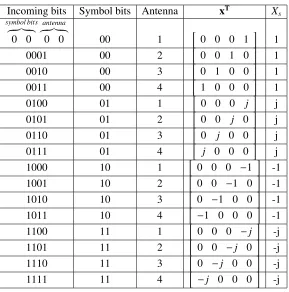
Table 2.1: SM scheme, Mapping input bits to corresponding constellation symbols and antenna space.

Incoming bits Symbol bits Antenna xT _X

s symbol bits

z }| { 0 0

antenna

z }| {

0 0 00 1 h 0 0 0 1 i 1

0001 00 2 h 0 0 1 0 i 1

0010 00 3 h 0 1 0 0 i 1

0011 00 4 h 1 0 0 0 i 1

0100 01 1 h 0 0 0 j i j

0101 01 2 h 0 0 j 0 i j

0110 01 3 h 0 j 0 0 i j

0111 01 4 h j 0 0 0 i j

1000 10 1 h 0 0 0 −1 i -1

1001 10 2 h 0 0 −1 0 i -1

1010 10 3 h 0 −1 0 0 i -1

1011 10 4 h −1 0 0 0 i -1

1100 11 1 h 0 0 0 −j i -j

1101 11 2 h 0 0 −j 0 i -j

1110 11 3 h 0 −j 0 0 i -j

1111 11 4 h −j 0 0 0 i -j

constellation symbol. This example requires two bits of input for the spatial domain and

an-other two bits for the constellation symbol ( which results in transmission of 4 bits at each

transmission time). For the sake of illustration, assume the input bits in a particular

transmis-sion instant is 1110. Such an input can be further divided into 11 and 10 (as explained before).

The first part (11) is mapped to the antenna space and thus it activates the fourth antenna, which

is shown by color red. Notice that rest of the antennas are silent. The second part of the

in-put bits (10) is assigned to the constellation diagram, which correspond to the third symbol in

QPSK and is highlighted by color yellow in the Figure. As a result, the constellation symbol

corresponding to input 10 is transmitted over fourth antenna element.

Alternatively, Fig. 2.1c gives an example of another transmission instance, when the input

(22)

2.1.2 Multi-stream Generalized Spatial Modulation

As in the case of SSK and G-SSK, SM can be generalized to trigger 1 < Na < Nt antennas

and transmit more than one symbol at a given transmission attempt. As such, generalized

spatial modulation (G-SM) takes the advantages of conventional SM as well as benefiting from

diversity gain. It worth mentioning that, deciding on an appropriate number of active antennas

(Na) is an important factor as it brings a trade of between complexity and data rate. For the

purpose of illustration, notice that there are

          Nt Na          

different combinations to selectNaantennas

from the totalNttransmitters. On the other hand, consideringmbits to select a set of antennas

containingNaelements results in 2mchoices, which causes

                           M Na           2m                 

distinct options. As an

example, consider a system with 4 transmit antennas out of which only 2 active antennas are

required. Furthermore, assumem=2. In such an example, there exists

          4 2          

=6 sets including

two antennas among which only 2m = ₂2 = _{4 sets can be used for the transmission. This}

results in           6 4          

= 15 different combinations. Notice that, increasing the number of transmit

antennas dramatically enlarges the number of combinations, each with different performance

[13]. Therefore, to address the challenge of selecting the optimum set of antennas by a feasible

approach, that eliminates the exhaustive search over entire set of combinations, is vital and

subject of the next Chapter.

An example of G-SM bit mapping strategy from input bits to antenna space and symbol

constellation is tabulated in Table 2.2. In this example, two activated antennas out of four

transmit antennas are used to convey a QPSK symbol.

In addition to enhanced spectral efficiency, G-SM has another advantage over SM

trans-mission. Particularly, unlike SM, where number of transmit antennas has to be a power of two,

G-SM does not have any constraint in this regard.

In addition to SSK/G-SSK and SM/G-SM, there are other methods to spatially modulate

the signal while increasing the spectral efficiency. Examples of these methods are quadrature

(23)

mention-Table 2.2: G-SM scheme, Mapping input bits to corresponding constellation symbols and

an-tenna space,Nt =4, Na= 2,m= 2, QPSK.

Incoming bits Symbol bits Antennas xT _X

s symbol bits

z }| { 0 0

antenna index

z }| {

0 0 00 (1,2) √1

2

h

1 1 0 0 i 1

0001 00 (3,4) √1

2

h

0 0 1 1 i 1

0010 00 (2,3) √1

2

h

0 1 1 0 i 1

0011 00 (4,1) √1

2

h

1 0 0 1 i 1

0100 01 (1,2) √1

2

h

j j 0 0 i j

0101 01 (3,4) √1

2

h

0 0 j j i j

0110 01 (2,3) √1

2

h

0 j j 0 i j

0111 01 (4,1) √1

2

h

j 0 0 j i j

1000 10 (1,2) √1

2

h

−1 −1 0 0 i -1

1001 10 (3,4) √1

2

h

0 0 −1 −1 i -1

1010 10 (2,3) √1

2

h

0 −1 −1 0 i -1

1011 10 (4,1) √1

2

h

−1 0 0 −1 i -1

1100 11 (1,2) √1

2

h

−j −j 0 0 i -j

1101 11 (3,4) √1

2

h

0 0 −j −j i -j

1110 11 (2,3) √1

2

h

0 −j −j 0 i -j

1111 11 (4,1) √1

2

h

−j 0 0 −j i -j

ing that non of the aforementioned spatial modulation techniques requires any channel state

information at the transmitter.

In summary, deploying a MIMO system brings a number of challenges, some of which are

itemized as follows and can be eliminated by spatial modulation techniques:

• Transmission of multiple bit streams requires the inter- antenna synchronization at the

transceiver sides.

• Each RF chain consists of PA, which in turn is the most power hungry component of the

system. Therefore, as the number of RF chain increases, the energy and power-efficiency

decreases.

• Inter-channel interference, which is a result of conducting multiple antennas degrades

(24)

2.2 Detection Algorithms

While the benefits of MIMO systems are well known for the future communication systems,

yet another difficulty of MIMO systems arises at the receiver side during the signal detection.

In general, detection algorithms fall into two main categories, i.e., linear and non-linear

detec-tions, some of which are discussed in this Section.

2.2.1 Low-complex Suboptimal Linear Detection

Linear detection algorithms aim to detect all transmitted streams at once by reversing the effect

of channel. Nevertheless, detection of all streams together reduces the diversity order.

Zero Forcing (ZF) Detection Algorithm

In ZF detection algorithm, the received signal is multiplied by inverse of the channel matrix to

achieve

H−1y=x+H−1n. (2)

This equation can be further used to detect the transmitted signalx. In other words, the weight

matrix in ZF is defined as WZF = H−1. Notice that in some practical applications, different

number of antennas are located at the transmitter and receiver. In such cases, the inverse of the

channel matrix can be replaced by its psudo-inverse and thus

WZF =

HHH−1HH. (3)

It is also worth mentioning that, maximum ratio combining (MRC) approach is a spatial

case of ZF. In particular, in scenarios, where there are single transmit antenna and multiple

(25)

Minimum Mean Square Error (MMSE) Detection Algorithm

Considering the last term in (2), one can notice that when the channel is in deep fade, i.e.,

chan-nel coefficients are close to zero, noise component enhances and deteriorates the performance

of detection. Therefore, in order to alleviate noise enhancement, another approach has been

proposed to find the weight matrix at the receiver side, which is based on minimizing the mean

square error and can be written as

WM MS E = min

W E

n

kx−Wyk2o

=min

W E

n

(x−Wy)H(x−Wy)o.

Taking the derivative of the above equation with respect to Wand set it to zero results in the

WM MS Erepresented by

WM MS E =

HHH+N0I

−1

HH. (4)

2.2.2 Successive Interference Cancellation Detection

To further improve the detection performance with acceptable increase in complexity, a series

of linear detection algorithms can be deployed in a multi-stream communication systems. In

this approach, every stream is reduced from the received signal after being detected. This

method is well-known as successive interference cancellation (SIC). For the sake of illustration,

the block diagram of such an algorithm is shown in Fig. 2.2.

2.2.3 Optimal Maximum Likelihood Detection

Similar to SIC, maximum likelihood detection is a non-linear detection. Notice that likelihood

function of received signalyis defined as the following probability

P(y|H,x)= √ 1

2πN0

e

−||y−Hx||2

(26)

Figure 2.2: Successive interference cancellation approach [2].

in whichN0is the variance of noise. To detect the transmitted signal, likelihood function needs

to be maximized, which alternatively is equivalent to minimizing the following distance metric

ˆ

x=arg min

∀x

ky−Hxk2, (6)

for all possible constellation symbols.

Notice that although ML detection is computationally expensive (as it searches through

all possible constellations) in comparison with linear detection algorithms, implementation of

ML on SM (shown in Fig. 2.3) achives lower complexity compared to ML detection in spatial

multiplexing (SMX). To be more specific, MIMO-SM with ML detection has 200(Nt−1)/(2Nt+

1)% complexity reduction in comparison with ML detection in SMX with the same spectral

efficiency [3]. That means 40% and more than 66% complexity reduction for systems with two

(27)

Figure 2.3: Block diagram of SM transmission and ML detection structure [3].

2.2.4 Log-Likelihood Detection Algorithm

The above mentioned detection algorithms are known as hard decision algorithms.

Neverthe-less, in order to reduce the information loss, other detection algorithms have been proposed

based on soft information. An example of such an algorithm is log-likelihood ratio (LLR) [2].

In MIMO systems, it is convenient to deploy soft decision in two steps. In the first stage,

a linear decoder is deployed to separate different bit streams, each of which can be further

considered for LLR calculation. To illustrate, let us consider a received signal as

y =

h1· · ·hNt

x+n

= h1x1+· · ·+hNtxNt +n. (7)

Then, the received signal can goes through the linear combination (using wi) to separate the

i-th bit as

ˆ

xi = wiy

(28)

Notice that, as in the last Section,wiisi-th row of matrixWcorresponding to either MMSE or ZF. In (8), desired component, interference and noise component are

di = wihixi, (9)

Ii =

Nt

X

j=1, j_, i

wihjxj, (10) and

ni =win, (11) respectively. In addition, considering independent noise and interference, the overall undesired

signal is a zero mean Gaussian random variable with variance of

σ2 i =

Nt

X

j= 1, j_,i

wihj

2

E

xj

2

+kwik2σ2n. (12)

Therefore, the conditional probability of estimating the i-th symbol given the exact value is

obtained by

f ( ˆxi|xi)= 1

q

2πσ2 i

exp −|xˆi−di|

2

2σ2_i

!

. (13)

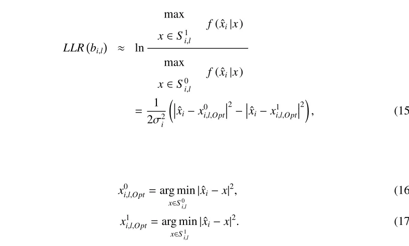
Assuming L-ary modulation, each symbol contains log₂(L) bits. Notice that, considering a

certain bit ini-th symbol, sayl-th bit (bi,l), theL-ary modulation space can be divided to two

subsets, i.e., those withbi,l = 0 and those withbi,l = 1, which can be represented byS0_i_,_l and

S1

i,l. As such, the LLR corresponding to thel-th bit ofi-th symbol can be evaluated as

LLR bi,l = ln P x∈S1

i,l

f ( ˆxi|x) P

x∈S0

i,l

f ( ˆxi|x)

(29)

which can be approximated as

LLR bi,l ≈ ln

max

x∈S1_i_,_l

f( ˆxi|x) max

x∈S0_i_,_l

f( ˆxi|x)

= 1

2σ2_i

xˆi−x

0 i,l,Opt

2

−

xˆi−x

1 i,l,Opt

2

, (15)

where

x0_i_,_l_,_Opt =arg min x∈S0

i,l

|xˆi− x|2, (16)

x1i,l,Opt =arg min x∈S1_i_,_l

|xˆi− x|2. (17)

Based on above equations and for the sake of illustration, we consider a 2×2 MIMO system

and evaluate the performance of LLR detection for different spectral efficiencies, namely, 8

bpcu and 4 bpcu. The results of Monte Carlo simulation is depicted in Fig. 2.5. We consider

the convolutional code with coding rate of 1/2, with block diagram shown in Fig. 2.4.

The channel is assumed to follow Rayleigh distribution and the Viterbi algorithm has been

deployed at the receiver with trace-back length of 32. These parameters are summarized in the

Table 2.3.

Table 2.3: Simulation parameters.

Parameter Value

Nt 2

Nr 2

Coding rate 1/2

Coding scheme Convolutional code

Trace back length for Viterbi algorithm 32

Polynomials 1111001=171(Oct)

(30)

Figure 2.4: Convolutional encoder with coding rate of 1/2 [4].

0 5 10 15 20 25 30

SNR(dB)

10-3 10-2 10-1 100

Average bit error rate

2 2 MIMO, 16QAM 2 2 MIMO, 4QAM

(31)

2.2.5 Performance Analysis of SM with Di

ff

erent Detection Algorithms

As explained earlier, in SM, as opposed to the conventional MIMO systems, a single antenna

is activated and the index of transmit antenna is used for the sake of information transmission.

As a result, one RF chain is needed. Thanks to single RF chain requirement, energy efficient

SM is a promising communication technology for future green transmission systems [1]. It is

also worth mentioning that in conventional MIMO systems, number of receive antennas needs

to be greater than those in transmitter, so that we can be able to apply MMSE or ZF.

Never-theless, as in the future wireless communication systems (such as in massive MIMO), where

number of transmit antennas is dramatically larger than number of receive antennas

(consider-ing downlink), SM becomes more favorable [3]. In addition to energy efficiency, SM reduces

the detection complexity. Maximum likelihood, which is known for its optimality and has

been proposed in [14], reduces the detection complexity fromO(MNt) in MIMO multiplexing

toO(MNt) in SM (assumingNt transmit antennas and constellation size ofM). Other types of

sub-optimal detection algorithms for SM-MIMO have been proposed, which further reduces

the complexity. Among all suboptimal detection approaches, [15] has proposed the separate

detection of the index information and symbol constellation and has become one of the most

important approaches. This separation and the fact that only a single antenna is activated allows

us to take advantage of simple MRC approach. As a result, the detection complexity reduces

toO(Nt+M).

In this section, we consider the performance of SM and compare the results with SMX

transmission having the same spectral efficiency. Notice that in SMX different antennas

trans-mit different bit streams and thus number of RF chains is equal to number of transmit antennas.

Let us start with the optimum detection algorithm, i.e., ML detection. In SM, the receiver uses

the ML to jointly detect the transmitted symbol as well as antenna indices.

We have made the comparison for different spectral efficiencies, i.e., R=6 and 10 bits per

channel use (per subcarrier), which have been shown in Fig. 2.6 and Fig. 2.7, respectively. In

SMX, we consider MIMO configuration with 2 antennas at the transmitter and receiver sides

and the performance has been depicted with black line while different MIMO configurations

(32)

0 5 10 15 20 25 30

SNR(dB)

10-5 10-4 10-3 10-2 10-1 100

2 2 SMX, 8PSK, R=6 2 2 SM, 32-QAM, R=6 4 2 SM, 16-QAM, R=6 8 2 SM, 8PSK, R=6

Figure 2.6: Comparison of spatial multiplexing and spatial modulation, 6 bits/subcarrier.

0 5 10 15 20 25 30

SNR(dB)

10-3 10-2 10-1 100

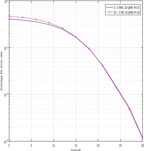
2 2 SMX, 32-QAM, R=10 32 2 SM, 32-QAM, R=10

(33)

Considering spectral efficiency of 6, (Fig. 2.6), simulation results show that increasing the

number of antennas, while utilizing a single RF chain, SM outperforms the MIMO system with

SMX transmission. Likewise, for higher spectral efficiency, i.e., R=10 bpcu shown in Fig. 2.7,

large number of antennas enables SM to achieve the performance of SMX while benefiting

from low cost and power efficient implementation.

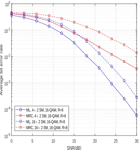
Fig. 2.8 shows the performance of SM in terms of ABER based on MRC detection and its

comparison with ML algorithm. Notice that, in SM with MRC algorithm, detection of

constel-lation symbols depends on the estimation of activated antenna index and thus if the antenna

index is detected erroneously, the symbol estimation would be highly incorrect. This results

can be seen in Fig. 2.8, where the joint detection of antenna index and symbol constellation,

i.e., ML detection, outperforms the MRC approach.

0 5 10 15 20 25 30

SNR(dB) 10-5

10-4 10-3 10-2 10-1 100

ML, 4 2 SM, 16-QAM, R=6 MRC, 4 2 SM, 16-QAM, R=6 ML, 16 2 SM, 16-QAM, R=8 MRC, 16 2 SM, 16-QAM, R=8

Figure 2.8: Comparison of MRC and ML detection of SM.

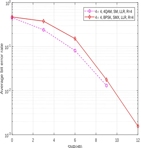
Finally, we have made the comparison of SM and SMX with LLR detection. Two different

MIMO configurations are shown in Fig. 2.9 and Fig. 2.10. Comparing two aforementioned

Figures, one can see that for the same spectral efficiency, increasing the number of antennas

(34)

0 2 4 6 8 10 12 14 16 18 20 SNR(dB)

10-3 10-2 10-1 100

2 2, 8QAM, SM, LLR, R=4 2 2, 4QAM, SMX, LLR, R=4

Figure 2.9: 2×2 SM-MIMO and SMX comparison based on LLR detection,R=4.

0 2 4 6 8 10 12

SNR(dB) 10-3

10-2 10-1 100

4 4, 4QAM, SM, LLR, R=4 4 4, BPSK, SMX, LLR, R=4

(35)

Antenna Selection in Dual-Polarized

Generalized Spatial Modulation

3.1 Introduction

The anticipated 1,000 times of dramatic capacity increase in 5-th generation (5G) wireless

networks has created many fundamental challenges. To meet the network capacity of 5G,

mas-sive multiple-input multiple-output (MIMO), which utilizes antenna array with a large number

of elements, has been widely considered as a critical enabling technology for 5G due to its

advantage of significantly increased spatial frequency reuse factor through the beamformed

spatial transmission. However, the number of RF chains (which dominates the implementation

cost of MIMO systems), needs to be equal to the number of antennas in conventional MIMO

systems. Consequently, this requirement will drastically increase the implementation cost of

massive MIMO systems due to a large number of antennas involved. As an alternative,

spatial-modulation emerges as one promising solution to benefit from a large number of antennas

while having limited number of RF chains, without sacrificing the data rate.

Spatial modulation (SM) is a relatively new transmission scheme, which uses the space

dimension of antenna array to convey part of the bit stream to be transmitted [12]. In

partic-ular, part of the input bits is used to select an antenna to be activated while the other part is

mapped onto the symbol that is transmitted through the selected antenna. Moreover, while SM

is deployed over the MIMO systems, it uses only one activated antenna, which significantly

(36)

reduces the complexity of the transceivers.

During the recent years, SM is widely considered in literature and its potential benefits

and challenges are evaluated [1]. The advantages of SM in large-scale MIMO systems is

considered in [16]. In addition, the gain achieved by antenna selection in SM is addressed

in [17] considering Euclidean distance and capacity of the system, while in [18], the authors

use circle packing algorithm to maximize the minimum geometric distance between antennas

to minimize the average bit error probability (ABEP) of SM-MIMO. Note that SM is a special

case of generalized SM (GSM), where more than one antenna are used to convey the bit stream

[19, 20]. As indicated in [21], as the number of transmit antennas increases, GSM outperforms

the conventional SM and therefore is preferable in massive MIMO. Nevertheless, the authors in

[13] show that the performance of GSM varies depending on the different antenna grouping and

not all of the antenna combinations benefit from sufficiently low ABEP. However, selecting an

antenna group which results in the best performance using the exhaustive search is intractable.

Therefore, to fill this gap, we present a novel and direct antenna grouping in GSM and remove

the necessity of search.

On the other hand, the performance of GSM-MIMO systems deteriorates substantially with

increased correlation among antennas due to insufficient inter-antenna spacing. In other words,

to have adequate uncorrelated channels, antennas should be implemented in the order of half

of the wavelength away from each other. However, by increasing the number of antennas in

large-scale MIMO systems, this space requirement cannot be met with the space constraint of

the transceivers. In addressing this, one promising approach to cope with the space limitation

is to use dual-polarized (DP) antennas [22–26]. Two orthogonal polarizations can be utilized

to differentiate the channels and impose an additional correlation due to the polarization

mis-match. The aforementioned correlation is known as cross-polar discrimination (XPD) and its

impact on the performance of antenna selection is considered in [27]. To take advantage of

DP-MIMO, while exploring the space dimension and benefiting from the performance of the

best antenna groups in GSM, we analyze a novel method to directly determine the optimum

antenna groups in DP-GSM.

The overall contributions of this Chapter are as follows: We analyze a MIMO system

(37)

GSM scheme, we propose a two-stage algorithm to determine the optimum antenna groups and

activate antennas within each group. In the first stage, we develop the procedure of selecting

a representative antenna and its polarization for each group. In the second stage, we establish

an algorithm to select antennas within each group to benefit from the advantages of GSM. We

use the average bit error probability (ABEP) of the system to evaluate the performance of the

proposed scheme and validate it by making a comparison with ABEP of the optimum antenna

grouping in DP-GSM, which is obtained by the exhaustive search. In addition, we compare the

performance of the proposed antenna grouping in DP-GSM system with the optimum

perfor-mance of the system with uni-polarized (UP) antennas, whose number of antennas are twice as

many as that of DP-MIMO.

The Chapter is organized as follows: In Section II, we introduce the system model and

characteristics of the DP channel. The proposed algorithm on DP GSM is provided in Section

III followed by the performance analysis in Section IV. We present the simulation results in

Section V and conclude the Chapter in Section VI.

3.2 System Model

We consider a MIMO system withNt and NrDP antennas at transmitter and receiver,

respec-tively, which leads to a 2Nt×2Nr dimensional channel between transmitter and receiver. We

useNt DP antennas to transmitm+`bits at each transmission instance. Therefore, the spectral

efficiency of such a system isR = m+` bits per channel use (bpcu). In other words, at each

transmission instant, m+` bits are chosen from the incoming bit stream. ` bits are mapped

onto theL-ary symbol space, where L=2`andX=

X1, . . . Xk, . . . XL

represents the

set of constellation symbols. The other m bits are used to select one antenna group

contain-ing Na antennas. In this work, we do not consider mapping optimization and therefore, both

bit-to-antenna and also bit-to-symbol are uniformly mapped. Notice that the transmitted signal

can be represented by a 2Nt ×1 vectorxu,s, whose entries are 0 in all butNa positions, which

denote the indices of activated antennas inuth group. We assume that allNaactivated antennas

transmit the same symbols ∈Xand therefore, the values of all non-zero elements of transmit

(38)

constraint of unity for transmitted signal, i.e.,Ex h

xu,sHxu,s= 1 i

.

The transmit signal vector,xu,s, is then transmitted over a DP-MIMO channel and received

by an array of 2Nrantennas as

y= √1

Na

Hxu,s+ν (1)

where division by √Na is for the purpose of power normalization. y andν are the 2Nr ×1

vectors representing received signal and channel noise, respectively. The elements of ν are

independent identically distributed (i.i.d.) complex Gaussian variables with zero mean and

varianceN0, i.e.,νk ∼ CN(0,N0) fork= 1, . . . ,2Nr, thus signal to noise ratio (SNR) is defined

byS NR = η = Es

N0 =

1

N0. Hrepresents the 2Nr×2Nt channel matrix between transmitter and

receiver whose elements are possibly correlated complex Gaussian random variables. Unlike

uni-polarized antennas, correlation in MIMO channel with DP antennas includes the

polar-ization effects within each DP antenna as well as spatial correlation due to the insufficient

space between antennas. To shed lights on the impact of different correlation matrices, we first

consider the single DP antenna at transmitter and receiver, which is also known as two-input

two-output (TITO) system in the following subsection and exhibit the effect of polarization

correlation. Consequently, we extend the TITO to MIMO scenario and present the impact of

spatial correlation.

3.2.1 TITO Scenario

We consider a TITO system, where only one dual-polarized antenna is deployed at the

trans-mitter and receiver. Therefore, the equivalent channel His a 2 ×2 matrix. If the channel is

not rich enough to adequately distinguish different polarizations, the channel would be affected

by the polarization correlation (XPC) between orthogonal polarization directions. However, as

stated in [28], the polarization correlations are small can be ignored in calculations for the sake

of simplicity. However, we consider it in our analytical derivations. The effect of polarization

correlation in transmitter and receiver can be represented in matrix form as

Πt =          

1 γt

γ∗ t 1          

, Πr =          

1 γr

(39)

respectively, where

γt =

Enhip,iph

∗ ip,ip0

o

p

µ(1−µ) =

Enhip0,iph

∗ i_p0,i_p0

o

p

µ(1−µ) ,

γr =

Enhjp,jph

∗ jp0,jp

o

p

µ(1−µ) =

Enhjp,jp0h

∗ jp0,jp0

o

p

µ(1−µ) ,

and 0 < µ ≤ 1 represents the amount of power leakage from one polarization to the other. In

other words,

µ = E

hip,ip0

2 =E hip0,ip

2

, (3)

where hip,ip0 represents the channel coefficient between ith antenna with pth polarization and

ith antenna with its orthogonal polarization,p0. Similarly, the rest of the power is expressed as

1−µ = E

hip,ip

2 = E hip0,ip0

2

. (4)

The power ratio of co-polar to cross polar terms are characterized by XPD as described in [24]

and shown by

χ= 1−_µµ. (5)

The amount of XPD is proportional to the capability of the channel to distinguish between the

two polarization directions.

3.2.2 MIMO Scenario

In this part, we consider the more general case with Nt and NrDP antennas at the transmitter

and receiver, respectively. Accordingly, the spatial correlation between antennas due to the

insufficient spacing of antennas at transmitter and receiver can be represented in a matrix form,

Σt and Σr, respectively. Notice that the correlation between separated antennas

(40)

amongith and jth antenna can be calculated as in [18] [Σt]i,j =α

di,j

t (6)

where|αt|< 1 anddi,jdenotes the distance betweenith and jth antennas.

Considering the effects of polarization correlation and spatial correlation, the generalized

2Nr×2Nt dual-polarized channel matrix can be written as [24]

H= 1Nr×Nt ⊗Γ

Ψ

r

1

2H

wΨt

1

2 (7)

whereΓis the leakage matrix which can be written as

Γ=           p

1−µ √µ

√

µ p

1−µ

          . (8)

The operatordenotes the element-by-element Hadamard multiplication. Hwis the size 2Nr×

2Nt matrix modelling the fading part of the channel. The elements of Hw are independent

and identically distributed (i.i.d.), circularly symmetric zero mean complex Gaussian variables

with unit variance. 1Nr×Nt is an all oneNr× Nt matrix and⊗denotes the Kronecker products.

Finally, it can be shown thatΨr =Σr⊗ΠrandΨt =Σt⊗Πt.

In order to adopt the antenna configuration as in [18], we assume the number of DP transmit

antennas is a power of 2, i.e., log₂(Nt) is an integer. We assume the antennas are located in a

square manner, where the number of antennas,A, in each edge of the square can be calculated

as in [18] given by

A=          √

Nt if log₂(Nt) is even

3×

q Nt

8 if log2(Nt) is odd.

(9)

Notice that when the log₂(Nt) is an odd number, Ainner =

q Nt

8 antennas (located at the center

of the square) are removed. Fig. 3.1 demonstrates the antenna configuration when number of

(41)

(a) (b)

Figure 3.1: DP antenna configuration with different number of antennas, a)Nt = 8 DP

anten-nas, b)Nt =4 DP antennas.

3.3 Proposed Antenna Grouping

In this section, we present the antenna grouping in DP-GSM MIMO systems and deduce the

framework to selectNaantennas within each group. In this regard, first we discuss the selection

of antennas together with their polarization, which are representative of different group.

Con-sequently, we consider the selection ofNaantennas within each group. Finally, the tractability

of the algorithm is compared with exhaustive search over all possible combinations of antenna

groups.

3.3.1 Selection of Group Indicators

Consideringmbits to select a group containingNaantennas as mentioned earlier, is equivalent

to having 2m_{groups of antennas. As stated in [18], the optimum performance in terms of ABEP}

can be achieved when these groups are chosen such that the correlation between them is low.

Nevertheless, unlike the uni-polarized system in [18] and as stated earlier in Section II, MIMO

systems with DP antennas are influenced not only by the spatial correlation but also by the

polarization correlation. As the polarization correlation is usually low [28] and thus ignorable,

the lowest correlations are among those antennas which have the most distance from each

other in geometrical point of view, while having orthogonal polarizations. In order to be able

(42)

indicators to follow the circle packing algorithm as in [18]. However, notice that adjacent

groups suffer from more spatial correlations. Therefore, to reduce the overall correlation we

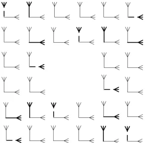
use different polarization from one group to its adjacent ones. For the sake of illustration, Fig.

3.2 presents an example of group’s indicators (including antenna location and its corresponding

polarization) by bold dashed lines. In this example, number of transmit DP antennas is 32, i.e.,

Nt =32. In addition, we assume the number of bits assigned to select a group is 3 (i.e.,m= 3),

which is equivalent to 23 = 8 groups of antennas.

3.3.2 Selection of Inner Group Antennas

Notice that there are Na antennas to be activated within each selected group. Therefore, we

suggest to select the Na antennas in each group in such a way that they are highly correlated

so that the overall correlation between different groups remains in its minimum level.

Con-sidering the fact that less spatial distance impose more spatial correlation among antennas and

as arrays with similar polarizations are impacted by higher polarization correlation, we select

Naantennas within each group as those which are close in terms of geometrical distance while

having the identical polarizations as those of the indicators . In Fig. 3.2 the activated antennas

in each group are shown as solid bold lines. We assume,Na= 2.

3.3.3 Feasibility of the Algorithm

In this Section, we evaluate the feasibility of the proposed algorithm and compare it with

the size of search space when considering the exhaustive search to find the optimum groups

of antennas to be activated. We illustrate the size of search space in exhaustive search via

an example. Suppose there are Nt antennas at the transmitter and Na activated antennas are

used to convey the information symbols. Therefore, there are

          Nt Na          

different combinations

of antennas. In addition, m bits from input bit stream being mapped to the antenna space is

equivalent to selection of 2m_{groups of antennas out of the total}

          Nt Na          

(43)

Figure 3.2: An example of antenna grouping considering their distance and polarizations,

as-sumingNt =32 DP antennas,m=3, andNa =2.

the search space of

                           Nt Na           2m                 

different combinations. Table 3.1 shows size of the search space

whenNt =16, and for different values ofNaandm.

m\Na 2 3

1           16 2 ! 2           = 7140           16 3 ! 2           =156520 2           16 2 ! 4           =8214570           16 3 ! 4          

>4×109

3           16 2 ! 8          

>8×1011

          16 3 ! 8          

>8×217

Table 3.1: Size of the search space for different values ofNa andm.

(44)

The large size of the search space in exhaustive search makes it intractable and highlights the

importance of proposed scheme. Unlike in exhaustive search, the proposed method directly

select the groups and antennas within each group together with their polarizations as explained

in Section II (sub-section A and B) and illustrated in Fig. 3.2. Consequently, the proposed

approach totally eliminates the search requirement.

Notice that Na = 1 is a special case indicating the conventional spatial modulation. In

such case, the proposed scheme reduces the dual-polarized version of the algorithm presented

in [18] which still requires following the polarization switch from one activated antenna group

to its adjacent groups.

3.4 Performance Analysis

To evaluate the accuracy of the proposed scheme, we consider the average bit error probability

(ABEP) using the well-known upper bounding relation of [29] as

¯

Pb≤ 1 2R

2m

X

u=1 2m

X

ˆ u=1

L X

s=1 L X

ˆ s=1

N(u,uˆ,s,sˆ)

R P¯s(u,uˆ,s,sˆ) (10)

where,Ris the spectral efficiency as defined before. N(u,uˆ,s,sˆ) is the number of bits in error

between the respective channel/polarization and symbol index pairs, and ¯Ps(u,uˆ,s,s) is the

corresponding average pairwise symbol error probability (APEP). Notice that each APEP is

expressed as

¯

Ps(u,uˆ,s,sˆ)= E       Q        r

kzk2 2               (11)

where z = √ 1

N0Na(Hxu,s −Hxuˆ,sˆ). For the sake of simplicity in the analytical derivation, we

alternatively represent thezvector in vectorized form as

z = √ 1

N0Na

Υvec 1Nr×Nt ⊗Γ

Ψ1₂

vec(Hw)

= √ 1

N0Na

Υdiag

vec 1Nr×Nt ⊗Γ

Ψ1 2vec(H

w)

(45)

whereΥ = xu,s−xuˆ,sˆ⊗IandΨ = ΨTt ⊗Ψr. As stated in [13], it can be shown thatzforms

a proper complex Gaussian random vector with its mean vector0and covariance matrix ofΛz

expressed as

Λz =

1

N0Na

ΥΓ0_ΨΓ0†_Υ†

(13)

whereΓ0 = diag

vec 1Nr×Nt ⊗Γ anddiag{.}represents a diagonal matrix. As given in [30],

the APEP in (9) can be computed by

¯

Ps(u,uˆ,s,sˆ)= 1

π

Z π₂

0

Λz

4 sin2θ+I

−1

dθ. (14) Once each APEP term is computed via (14) the ABEP in (10) can be obtained conveniently.

3.5 Simulation Results

In this section, we present simulation results to evaluate the performance of the proposed

an-tenna grouping scheme in DP-GSM systems. To this end, we consider the derived ABEP in

the last Section. We assumeNt =8 andNr =1 DP transmit and receive antennas, respectively.

we assumeγ = 0.1, as larger values usually are not considered [24]. All Figures provide the

simulations for the scenarios when there are low and high spatial correlations among transmit

antennas. In all Figures, two sets of curves represent the performance of the system with low

spatial correlation between transmit DP antennas (depicted by the solid lines) and the highly

correlated DP antennas at the transmitter (dashed lines). In all simulations, we assumeαt = 0.1

for low spatial correlation and αt = 0.8 when the transmit DP antennas are highly correlated.

In all Figures and for both set of curves, we compare the performance of the proposed

algo-rithm and compare it with the best and the worst performances, which are obtained based on

exhaustive search. Thus for the sake of comparison and to achieve antennas which result in

the best and worst ABEP performances, we have evaluated the analytical derivations at a fixed

SNR, i.e., SNR=30 dB and consider exhaustive search (ES) over all possible antenna groups.

To this end and to be able to do the comparison, i.e., to make the exhaustive search tractable(

(46)

In Fig. 3.3 we assume two antennas are used (Na = 2) to transmit a QPSK and 8-PSK

symbols in different subfigure, i.e. R=3 and 4 bpcu in partaandb, respectively. Likewise, in

Fig. 3.4, we consider 3 activated antennas (Na= 3) conveying QPSK and 8-PSK constellations

in part a and b, respectively. The results indicate the tight match of the proposed antenna

grouping algorithm with the best performance. All simulated performances are compared with

the ABEP upper bounds; in the Figures, the simulated BER results are depicted only with the

markers while the ABEP upper bounds are plotted with lines.

In addition, we compare the proposed method in DP-MIMO with the best performance of

the equivalent channel with uni-polarized (UP) antenna elements. We use exhaustive search

to find the antenna groups which results in the best ABEP. Notice that the number of physical

channels in Nt × Nr DP-MIMO is equivalent to the those of the system with 2Nt ×2Nr

uni-polarized (UP) arrays. More specifically, we evaluate the performance of 16× 2 UP-MIMO

and compare it with 8×1 DP-MIMO. Notice that, since we consider the same antenna

con-figuration as in [18], 16 UP antennas occupies 4/3 more space in each edge of the square. In

other words, each edge contains 4 antennas in UP scenario while 3 DP antennas in DP-MIMO

systems. We make the comparison in both cases of low and high correlated antennas. The

per-formance of the UP-MIMO in Fig. 3.3 and Fig. 3.4 are depicted by bold lines. Notice that low

and high correlations between antennas indicate the inter-antenna spacing is large and small,

respectively.

As shown in the Figures, in low correlation channels, DP-GSM suffers for about 3 dB

performance loss while benefiting from the compact implementation. The advantages of

DP-GSM is more highlighted in high correlated channels. Notice that in practice, antennas are

implemented closed to each other (due to the space limitation), which impose higher

correla-tion between antennas. In this scenario, DP-GSM reaches the performance of UP-GSM and

yet take the advantage of close-packed deployment. These observations together with search

elimination to find the optimum antenna groups highlights the importance of the direct antenna

(47)

3.6 Conclusion

In this Chapter, we use antenna polarization to differentiate different channels while

achiev-ing compact implementation of wireless transceivers with multiple antennas. We propose a

two-stage antenna grouping scheme in generalized spatial modulation MIMO systems with

dual-polarized antennas, which leads to the lowest possible ABEP (optimum performance).

This algorithm directly selects the groups and activated antennas within each group, thus

elim-inating the requirement of searching for the groups with the best ABEP performance. The

ABEP performance of the proposed algorithm is validated by Monte Carlo simulations. We

also compare the ABEP of the proposed antenna grouping in DP-GSM with the optimum

an-tenna groups which are obtained by exhaustive search and the results from the two methods

are tightly matched. In addition, the simulation results validate the importance of the

algo-rithm to optimally group the antennas in DP-GSM as compared to UP-GSM. In particular,

when the channel is high correlated, the proposed method for DP-GSM reaches the optimum

performance of the UP-GSM with a twice as many as antennas in DP-MIMO. In low

correla-tion channels, DP-GSM is preferable in terms of physical space while suffering for about 3 dB