Data–Driven Fault Diagnosis of a Wind Farm
Benchmark Model
Silvio Simani1,∗, Paolo Castaldi2and Saverio Farsoni1
1Dipartimento di Ingegneria, Università degli Studi di Ferrara. Via Saragat 1E, Ferrara (FE) 44122, Italy;
{silvio.simani,saverio.farsoni}@unife.it
2Dipartimento di Ingegneria dell’Energia Elettrica e dell’Informazione “Guglielmo Marconi” – DEI, Alma Mater
Studiorum Università di Bologna. Viale Risorgimento 2, 40136, Bologna (BO), Italy. [email protected] * Correspondence: [email protected]; Tel.: +39-0532-97-4844
Abstract:The fault diagnosis of wind farms has been proven to be a challenging task and motivates the research activities carried out through this work. Therefore, this paper deals with the fault diagnosis of a wind park benchmark model, and it considers viable solutions to the problem of earlier fault detection and isolation. The design of the fault indicator involves data–driven approaches, as they can represent effective tools for coping with poor analytical knowledge of the system dynamics, noise, uncertainty and disturbances. In particular, the proposed data–driven solutions rely on fuzzy models and neural networks that are used to describe the strongly nonlinear relationships between measurement and faults. The chosen architectures rely on nonlinear autoregressive with exogenous input models, as they can represent the dynamic evolution of the system along time. The developed fault diagnosis schemes are tested by means of a high–fidelity benchmark model, that simulates the normal and the faulty behaviour of a wind farm installation. The achieved performances are also compared with those of a model–based approach relying on nonlinear differential geometry tools. Finally, a Monte–Carlo analysis validates the robustness and the reliability of the proposed solutions against typical parameter uncertainties and disturbances.
Keywords: fault diagnosis; analytical redundancy; fuzzy logic; neural networks; data-driven approaches; nonlinear geometric approach; wind farm benchmark simulator
1. Introduction
The increased level of wind–generated energy in power grids worldwide raises the levels of reliability and sustainability required of wind turbines. Wind farms should have the capability to generated the desired value of electrical power continuously, depending on the actual wind speed level and on the grid demand.
As a consequence, the possible faults affecting the system have to be properly identified and treated, before they endanger the correct functioning of the turbines or become failures. Wind turbines in the megawatt size are extremely expensive systems, therefore their availability and reliability must be high, in order to assure the maximisation of the generated power while minimising the Operation and Maintenance (O & M) services. Alongside the fixed costs of the produced energy, mainly due to the installation and the foundation of the wind turbine, the O & M costs could increase the total energy cost up to about the 30%, particularly considering the offshore installation [1].
These considerations motivate the introduction of fault diagnosis systems that can be also coupled with fault tolerant controllers [2,3]. Actually, most of the turbines feature a simply conservative approach against faults that consists in the shutdown of the system to wait for maintenance service. Hence, effective strategies coping with faults have to be studied and developed, for improving the turbine performance, particularly in faulty working conditions. Their benefits would concern the prevention of failures that jeopardise wind turbine components, thus avoiding unplanned replacement of functional parts, as well as the reduction of the O & M costs and the increment of the energy production. The advent of computerised control, communication networks and information techniques
brings interesting challenges concerning the development of novel Fault Detection and Diagnosis (FDD) and Fault Tolerant Control (FTC) design strategies for industrial processes.
Indeed, in the recent years, many contributions have been proposed related to the topics of fault diagnosis of wind turbines and wind farms, seee.g.[4,5]. Some of them highlight the difficulties to achieve the diagnosis of particular faults,e.g. those affecting the drive–train, at wind turbine level. However these fault are better dealt with at wind farm level, when the wind turbine is considered in comparison to other wind turbine of the wind farm [2]. Moreover, fault tolerant control of wind turbines has been investigatede.g.in [3,6] and international competitions on these issues arose [7,8].
Therefore, the fault diagnosis of wind turbine and wind farm systems has been proven to be a challenging task and motivates the research activities carried out through this paper.
In recent years, the increasing demand for energy generation from renewable sources has led to a growing attention on wind turbines. Indeed, they represent very complex systems which require reliability, availability, maintainability, safety and, above all, efficiency on the generation of electrical power. Thus, new research challenges arise, in particular in the context of modelling and control. Advanced control systems can also provide the optimisation of energy conversion and guarantee the desired performances even in presence of possible anomalous working condition, caused by unexpected faults and anomalous working conditions.
This work deals with the fault diagnosis of a wind farm system, and it proposes the application of viable and reliable solutions to the problem of earlier Fault Detection, Isolation (FDI) and estimation. Further fault tolerant controllers, which are not considered in this work, can be based on the fault diagnosis module developed in this paper, that provides the on–line information on the faulty or fault–free status of the system and the fault estimation, so that the controller action can be compensated. The design of the fault diagnosis system involves data–driven approaches, as they offer an effective tool for coping with a poor analytical knowledge of the system dynamics, noise, uncertainty and disturbance.
The first data–driven proposed solution relies on fuzzy Takagi–Sugeno models, which are derived from a clusteringc–means algorithm, followed by an identification procedure solving the noise–rejection problem. Furthermore, a second solution makes use of neural networks to describe the strongly nonlinear relationships between measurement and faults. The chosen network architecture belongs to the Nonlinear AutoRegressive with eXogenous (NARX) input topology, as it can represent a dynamic evolution of the system along time. The training of the neural network fault estimators exploits the classic back–propagation Levenberg–Marquardt algorithm, that processes a set of acquired target data.
A purely nonlinear model–based scheme for fault tolerant control purpose was also proposed by the same authors, which is based on NonLinear differential Geometric Approach (NLGA) tools [9]. Already suggested by the authors also in the aerospace framework [10], it was extended by the same authors to the active fault tolerant control for the same wind farm simulator [11], but it is considered here only for comparison purpose.
The developed fault diagnosis schemes are tested by means of a high–fidelity benchmark model, that simulates the normal and the faulty behaviour of the wind farm system. The performances achieved via the data–driven approaches are analysed and compared with the proposed nonlinear model–based approach. Moreover, a Monte–Carlo analysis validates the robustness and reliability features of the proposed fault diagnosis schemes against the typical parameter uncertainties and disturbances. Finally, the effectiveness shown by the obtained results suggests further investigations on the industrial application of the proposed fault diagnosis methodologies.
nonlinear FDD strategy is also reported. Finally, Section6concludes the paper by summarising the main achievements of the work, and providing some suggestions for further research issues.
2. Wind Farm Benchmark Model
The wind farm benchmark model considered in this monograph has been proposed in [2] by the same authors who developed the wind turbine benchmark model [3].
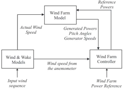
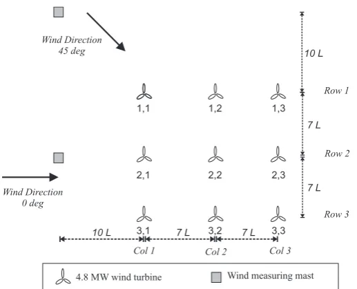
It consists of 9 wind turbines arranged in a squared grid of 3 rows and 3 columns. The complete wind farm model consists of 3 main submodels: the wind and wake model, the plant model, and the controller model, interacting as sketched in Figure1. The layout of the wind farm with 9 turbines of the square grid and the masts along the wind directions are sketched in Figure2.
Wind Farm Model
Wind & Wake Models
Wind Farm Controller
Wind speed from the anemometer Actual Wind
Speed
Reference Powers
Generated Powers Pitch Angles Generator Speeds
Input wind sequence
Wind Farm Power Reference
Figure 1.Block diagram of the wind farm benchmark model.
The distance between the wind turbines in both directions is 7 times the rotor diameter,L. Two measuring masts are located in front of the wind turbines, one in each of the wind directions considered in this benchmark model,e.g.0 deg and 45 deg. The wind speed is measured by these measuring masts which are located in a distance of 10 timesLin front of the wind farm. In this way, the measuring devices are not affected by the wind turbine wakes and are able to provide sufficiently accurate wind speed measurements. The wind turbines of the farm are defined by their row and column indices in the coordinate system, as illustrated in Figure2.
The farm uses generic 4.8 MW wind turbines, which are three–bladed horizontal–axis, pitch–controlled variable–speed wind turbines. Each of the wind turbines is described by simplified models including control logics, variable parameters and 3 states [2].
2.1. Wind and Wake Model
The wind and wake model provides the wind speed for each of the 9 turbines, contained in the vectorvw, as well as for a measuring mastvw,m. They are determined starting from a certain wind sequence (two different wind sequences are included in the simulator) and their elaboration takes into account the delay and the interaction among the turbines depending on wind direction. In particular, the wake effect is described as reported in [12] by means of a static deficit coefficient of 0.9. Finally the turbulence is modelled by an additive Gaussian white noise.
2.2. Wind Farm Benchmark Overall Model
1,1 1,2 1,3
2,1 2,2 2,3
3,1 3,2 3,3
Row 1
Row 2
Row 3
Col 1 Col 2 Col 3
10 L 7 L 7 L
7 L 7 L 10 L
Wind Direction 0 deg
Wind Direction 45 deg
4.8 MW wind turbine Wind measuring mast
Figure 2.Layout of the wind farm benchmark with 9 wind turbines.
Inside the turbine submodel, the current wind speed is elaborated by means of a look–up table in order to compute the available powerPw(t). Then, the generated power is computed according to the relation of Eq. (1):
Pg(t) =Pc(t) +γpsin(2πσpt) (1) where the first termPc(t)is equal to the current lower value between the filtered available power ˆPw and the filtered reference power ˆPr:
Pc(t) =
(
ˆ
Pw(t), if ˆPw(t)<Pˆr(t) ˆ
Pr(t), if ˆPw(t)>Pˆr(t) (2) The second term of the Eq. (1) represents the oscillations caused by the drive–train, whose amplitude isγpand frequencyσp.
The filtered signals ˆPw(t)and ˆPr(t)differs from the input variables by means of a first order transfer function in the form of Eqs. (3) and (4):
ˆ Pw(s) =
τw(vw) s+αw(vw)Pw
(s) (3)
ˆ Pr(s) =
τp s+τp Pr
(s) (4)
where the parameterτpis a fixed value, while the functions τw(·)andαw(·)depend on the wind speed and are computed by means of a look–up table. Note that descriptions using maps rather than analytical functions allow to provide a a computationally simple, but at the same time, also a realistic simulator of wind farm system. On the other hand, the relations of Eqs. (3) and (4) describe the filtering effect of the wind farm on the available and reference powers, respectively, which cannot change instantaneously.
The relation between the reference pitch signal and the actual pitch angle of the wind turbine of the wind farm has been described by a first–order transfer function in the form of Eq. (5):
β(s) = τβ
s+τβ
With respect to the second–order system already considerede.g.in [3], this means that the wind turbine blades of wind farm simulator are actuated by means of electric motors rather than hydraulic systems.
Then, the generator speed of each turbine is modelled as described in Eq. (6):
ωg(t) = fω(Pc(t))
1+ γp
ωg,max sin
(2π σpt)
(6)
where fω(·)is computed by means of a look–up table, whilst the oscillation term, due to the drive–train,
has an amplitude equal to the ratio between the parameterγpand the maximal generator speedωg,max. In this way, the relation of Eq. (6) allows to include both the generator controller and the effect of the drive–train oscillations, which depend on its time–constant 1/σpand the damping factorγp. This term is also reduced by the maximal generator speedωg,max.
Finally, the wind farm controller forces each turbine to follow a reference power signalPr(k)that is 1/9 of the wind farm power reference. Moreover, in order to avoid fast variation of the control signal, the wind farm power reference is low–pass filtered obtaining ˆPw f,r. The controller is modelled as discrete–time system and uses a sample frequency of 10 Hz [2]:
Pr(k) = 1
9Pˆw f,r(k) (7)
2.3. Wind Farm Fault Scenario and Model Parameters
3 common fault scenarios are considered [2]. They affect the output variables of the plant system. These kinds of fault are difficult to detect considering the single wind turbine, but they can be identified at wind farm level.
The first fault considered represents the debris build–up on the blade surface. Its effect corresponds to a change of the aerodynamic of the affected turbine and the consequent decreasing of the generated power that is modelled by a scaling factor of 0.97 applied to the generated power signal. An analysis of this kind of fault is reported in [13].
The second fault is a misalignment of one blade caused by an imperfect installation. The effect is an offset between the actual and the measured pitch angle of the affected turbine. This fault can excite structural modes and creates undesired vibrations that can damage the system severely. The faulty signal involves an offset of 0.3 deg on the pitch angle.
The third fault represents the wear and tear in the drive–train. It was demonstrated [7] that this kind of fault is difficult to detect at wind turbine level, and the current trend is to analyse the frequency spectra of different vibration measurement. In this benchmark model the fault affects the generated power increasing the amplitude of its oscillation of the 26% of the nominal value, and the generator speed increasing the amplitude of its oscillation of the 130%.
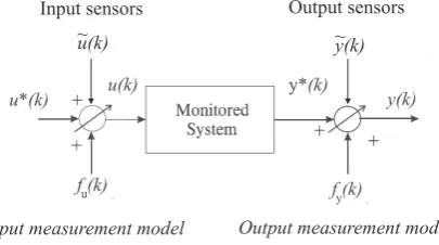
Table1summarises the considered faults, with a brief description of their typology and topology.
Table 1.The fault scenarios considered for the wind farm benchmark model.
Fault case Fault description Fault model Fault effect
1 Blade surface debris build–up Scaling factor (aerodyn. model) Reduced generated power 2 Blade misalignment Sensor offset Measured pitch angle offset 3 Drive–train wear and tear Drive–train model params. Generator speed oscillation
Finally, Table2reports the parameters used in the wind farm benchmark model.
3. Data–Driven Fault Diagnosis Strategies
Table 2.Parameter values of the wind farm benchmark model.
Variable name Parameter value
R 57.5m
τp 1.2rad/s
γp 1000W
σp 10Hz
τβ 1.6rad/s
ωg,max 158rad/s
3.1. Fault Diagnosis Scheme
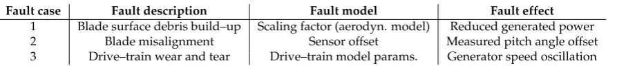
In the following the discrete–time monitored systems,i.e. the faults on the input and output measurements that are acquired from the wind farm simulator, as represented in Figure3, are described in the form of Eq. (8):
(
u(k) = u∗(k) +u˜(k) +fu(k)
y(k) = y∗(k) +y˜(k) +fy(k) (8) whereu∗(k)andy∗(k)are the actual unmeasurable variables, whilstu(k)andy(k)represent the sensor measurements, affected by both the measurement noise and the faults.fu(k)andfy(k)are additive fault signals, that assume values different from zero only in presence of faults. Note that these terms representequivalentfault signals that produce the same effects of the actual faults affecting the wind farm, as described in Section2.3.
The same considerations hold for the measurement noise or error signals ˜u(k)and ˜u(k). They are modelled as white Gaussian process additive noise terms on the actual measurements acquired from the process under investigation, and are equivalent signals representing the actual effect of the measurement errors. This representation is also known as Errors–In–Variables (EIV) model [14].
u(k) y(k)
Input sensors Output sensors
Input measurement model Output measurement model
~ ~
Figure 3.The equivalent fault and measurement error description of the system under diagnosis.
Figure3shows the general scheme with the faults affecting the system under diagnosis,i.e.the wind farm, as equivalent additive signals on the input and output measurements (sensors).
Among the different approaches to generate the residual signals available in the related literature, the solution proposed in this work exploits two approaches. They rely on fuzzy and neural network models, which provide on–line estimations of the fault signalsfu(k)andfy(k). Hence, as shown in Figure4, the residualsrare represented by the estimated fault signals ˆf(k)generated by the fault estimators filtering the measured (sampled) inputs and outputsu(k)andy(k), respectively:
r(k) =ˆf(k) (9)
Fault indicator
Input
sensors
Output
sensors
Wind farm simulator
Fault estimator
r(k) = (k)^f
u(k)
y(k)
y(k)
y(k)
u(k)
u(k)
~
f (k)
yy(k)
~
f (k)
uFigure 4.The general residual generation scheme relying on fault estimators.
Figure4sketches the residual generation scheme that is achieved via the fault estimator system, by using the acquired input and output measurementsu(k)andy(k). The fault diagnosis process requires, as first step, the FDI tasks. As the residual is equal to the estimated fault signal, it is easily performed here by using a proper thresholding logic directly operating on the residuals, without requiring their elaboration with any evaluation functions, as addressede.g.in [15]:
Therefore, the occurrence of thei–th fault can be simply detected via the threshold logic of Eqs. (10) applied to thei–th residualri(k):
(
¯
ri−δσri ≤ri≤r¯i+δσi fault–free case ri<r¯i−δσri orri>r¯i+δσri faulty case
(10)
where thei–th componentri(k)of the residual vectorr(k)of Eq. (9) is considered a random variable, whose unknown mean ¯riand varianceσr2i are estimated in fault–free condition, after the acquisition of
Nsamples, as shown by the relations of Eqs. (11):
(
¯
ri = N1 ∑Nk=1ri(k)
σr2i = N1 ∑Nk=1(ri(k)−r¯i)2
(11)
The tolerance parameterδhas to be properly tuned in order to separate the fault–free from the faulty
situations. Theδvalue determines the trade–off between the false alarm rate and the fault detection
probability. A common choice ofδcan rely on the three–sigma rule, otherwise extensive simulations
can be performed to optimise theδvalue.
Consequently to the fault detection, the fault isolation task is easily achieved by means of a bank of estimators. As described by Eqs. (8), the faults are considered as equivalent signals that affect the input measurements,i.e.fu, or the output measurements,i.e.fy.
Dynamic process
…
…
u (k)
…
u (k)…
u (k) 1 2 r y (k) y (k) y (k) 1 2 m
…
…
Fault estimator Fault estimator Fault estimator Fault estimator 1 2 i r+m Bus Bus Selector Selectoru (k)j
y (k)l
r (k) = f (k)
r (k) = f (k)
r (k) = f (k)
r (k) = f (k)
1 1 2 2 i i r+m r+m Selector Selector Selector Selector Selector Selector
Figure 5.The general estimator scheme for the reconstruction of theequivalentinput or output faults, fuorfu.
Figure5shows this generalised fault estimator scheme, where the fault estimators are driven only by the input–output signals selected via the FMEA tool addressed in Section3.2, so that the relative residualri(k) = fˆi(k)is insensitive only to the fault affecting those inputs and outputs defined by the selector blocks. It is worth noting that multiple faults occurring at the same time could be correctly isolated using this configuration, if the FMEA procedure is properly performed.
The capabilities of the adopted estimator banks can be summarised by means of the so–called fault signaturematrix, depicted in Table3, where each entry that is characterised by a value equal to ‘1’ means that the considered residual (i.e.the equivalent fault) is sensitive to the actual fault effect (‘0’ otherwise), under the hypothesis above mentioned.
Table 3.Fault signatures for the generalised fault estimator bank.
u1 u2 . . . ur y1 y2 . . . yr
r1 1 0 . . . 0 0 0 . . . 0
r2 0 1 . . . 0 0 0 . . . 0 ..
. . .. . . . ...
rr 0 0 . . . 1 0 0 . . . 0
rr+1 0 0 . . . 0 1 0 . . . 0
rr+2 0 0 . . . 0 0 1 . . . 0 ..
. . . .. ...
rr+m 0 0 . . . 0 0 0 . . . 1
As already remarked, the FMEA tool [16], that has to be executed before the design of the fault estimators, suggests how to select the input–output configuration for the fault estimator blocks. This input–output selection procedure, that is briefly remarked here, will be addressed in more detail in Section3.2. Then, the design of the fuzzy or neural network models can be performed, as recalled in Sections3.3and3.4, respectively. Finally, the threshold test logic of Eq. (10) allows the achievement of the fault diagnosis tasks.
3.2. Failure Mode & Effect Analysis for the Wind Farm System
measurements with respect to the simulated fault conditions. In practice, the monitored fault signals have been injected into the benchmark simulator, assuming that only a single fault may occur in the considered plant. Then, the Relative Mean Square Errors (RMSE) between the fault–free and faulty measured signals are computed, so that, for each faultfi(k), the most sensitive signals (uj(k)andyl(k)) to that specific fault are selected.
In particular, the FMEA is conducted on the basis of a selection algorithm that is achieved by introducing the normalised sensitivity functionNx, defined in the form of by Eq. (12):
Nx= Sx S∗
x
(12)
where:
Sx=
xf(k)−xn(k) 2
kxn(k)k2 (13)
S∗x=max
xf(k)−xn(k) 2
kxn(k)k2 (14)
Its value represents the effect of the considered fault case with respect to a certain measured signal x(k). The subscripts ‘f’ and ‘n’ indicate the faulty and the fault–free case, respectively. Therefore the measurements mostly affected by the considered fault imply a value ofNxequal to ‘1’. Otherwise, smaller values of Nx mean that the signal x is not practically affected by the fault. The signals characterised by the highest value ofNxcan be selected as the most sensitive measurements and they will be considered in the design of the fault diagnosis blocks.
The results of the FMEA sensitivity are reported in Table4for the wind farm benchmark. The selected signals for each fault included in the wind farm benchmark are divided as inputs and outputs.
Table 4.FMEA and selected benchmark signals.
Fault casefi(k) Most Sensitive Measurementsuj(k)andyl(k)
1 β2,Pg,2,β7,Pg,7,vw,m 2 β1,ωg,1,β5,ωg,5,vw,m 3 β6,Pg,6,β8,ωg,8,vw,m
As a result, the fault diagnosis blocks that are designed as shown in Figure 5 exploit the reduced subset of input and output signalsuj(k)andyl(k)of Table4, instead of using all the system measurements recalled in Section2.2. Moreover, this leads to a noteworthy simplification of the residual generator structure, thus providing also a decrease in the computational effort.
Finally, the threshold test logic of Eq. (10) allows the achievement of the fault diagnosis task. The design of the fuzzy systems and neural networks will be recalled in the next Sections3.3and3.4, respectively.
3.3. Fuzzy System Modelling
This section describes the design of the fault estimators that is achieved by means of Takagi–Sugeno (TS) prototypes [17]. Indeed, the unknown relationships between the measurements acquired from the wind farm simulator and the considered faults are described by fuzzy models. They consist of a number of rules connecting the inputs with the output of the system under diagnosis, on the basis of a knowledge of its dynamics in form of IF=⇒THEN relations, processed by fuzzy reasoning [18].
According to the TS modelling approach, the consequents become crisp functions of the input, while the antecedents remain fuzzy propositions, therefore the fuzzy rule takes the form of Eq. (15) [17]:
Ri: IF (fuzzy combination of inputs) THEN output=gi(inputs) (15) where i indicates the number of rules, withi = 1, . . . ,nC. The antecedent does not differ from the Mamdani rules, with a combined membership functionλi(x)that takes into account the logical connectives expressed by linguistic propositions. The rule consequent functionsgihave a defined structure: it is the instance of parametrised function in affine form:
hi=aTi x+bi (16)
whereaiis a parameter vector andbiis a scalar offset, whilehiis thei–th rule output. The number of rules is supposed equal to the number of clustersnCused for partitioning the data into regions where local affine relations can be assumed [18]. Furthermore, the antecedent of each rule defines the degree of fulfilment for the corresponding consequent model, so that the rule global model can be seen as a fuzzy composition of local affine models.
Thus, the TS inference takes the form of the simple algebraic expression of Eq. (17):
ˆ f = ∑
nC
i=1λi(x)hi
∑nC i=1λi(x)
(17)
According to this description, the estimated fault ˆf is the weighted average of affine functions of the measured input and output signals, where the weights are the combined degree of fulfilment of the system input and output measurementsu(k)andy(k).
It is worth noting that the nonlinear system under diagnosis has a dynamic behaviour: therefore, the considered model input vectorxcan contains the current as well as the previous samples of the process input and output measurementsu(k)andy(k).
Indeed, in order to introduce the time dependence into the model of Eq. (15), the consequents are considered as discrete–time linear AutoRegressive models with eXogenous input (ARX) of ordero, in which the regressor vector takes the form of Eq. (18):
x(k) = hyj1(k−1), . . . , yj1(k−o), . . . , yjl(k−1), . . . ,yjl(k−o), uh1(k), . . . , uh1(k−o), . . . ,uhp(k), . . . , uhp(k−o)
iT (18)
whereuhp andyjl are the actual system input and output vectors, whose subscript indicesjlandhp
depend on the FMEA selection procedure of Section3.2, with 1≤ jl≤mand 1≤hp≤m.kis the time step, withk=1, 2, . . . , N. The affine parameters of Eq. (16) can be grouped as in the expression of Eq. (19):
ai=hα1,(i)j
1, . . . , α (i)
o,j1, . . . ,α (i)
1,jl, . . . , α (i) o,jl,δ
(i)
1,h1, . . . ,δ (i)
o,h1,· · ·,δ (i)
1,hp, . . . , δ (i) o,hp
iT
(19)
where theα(si)coefficients are associated to the output samples, and theδq(i)are associated to the input ones.
Indeed, fuzzy clustering allows an item to belong to several cluster simultaneously, with different degrees of fulfilment, whereas the classic crisp clustering relies on mutual exclusive subsets. Different clustering methods have been proposed in literature, seee.g.the review [21], or more recent works [22,23].
Typically, the available data consist of noisy measurements acquired from the system under diagnosis. They are grouped into the data matrixZ, whose columns are the vectorszcontaining the measurements of a single observation of the monitored process:
Z=
z11 . . . z1N ..
. . .. ... zn1 . . . znN
(20)
wherenis the data dimension, andNis the number of available observations.
Most fuzzy clustering algorithms are based on the optimisation of thec–means goal function J(Z,U,V)performed as follows:
• the data matrixZof Eq. (20) is defined;
• the so–called fuzzy partition matrix U = [µik] is defined, which contains the values of the membership function for the couplei–th measurement/k–th cluster;
• the vector V = [v1, . . . ,vnC] containing the cluster prototypes is defined; they have to be
determined and represent the centres from which the distance of each measurement is computed.
The widespreadc–means goal function adopted in this work was formulated in [24] and defined in the form of Eq. (21):
J(Z,U,V) =
nC
∑
i=1 N
∑
k=1
(µik)mD2ikA (21)
m>1 being the weighting exponent, and:
D2ikA=kzk−vik2A= (zk−vi)TA(zk−vi) (22) the squared inner product distance norm, withi = 1, . . . ,nC and k = 1, . . . , N. The matrix A determines the cluster shape.
The minimisation algorithm exploits a series of Picard iterations that updates the cluster prototypesVand of the partition matrixU, until a stop criterion is met [18].
An important point concerns the determination of the optimal number of clustersnC, since the clustering algorithm assumes a suitable number of clusters, regardless of whether they are really present in the data or not. Once the partition matrixUhas been estimated, the antecedent degrees of fulfilmentµikinUare easily estimated by interpolation or curve fitting methods [18].
3.3.1. Fuzzy Model Parameter Estimation
In fact, the discrete–time dynamic model already represented in Figure3is considered in the EIV framework, the noise is supposed to affect the inputsuas well as the output measurementsyas additive signals ˜uand ˜yon the noise–free unmeasurable quantitiesu∗andy∗, in the form of Eq. (23):
(
u(k) = u∗(k) +u˜(k)
y(k) = y∗(k) +y˜(k) (23)
Therefore, by considering thei–th TS consequent of the type of Eq. (17) and the associated local ARX model of orderowith the regressors grouped into the vectorxas in Eq. (18), the acquisition ofNinoisy measurement of input and output samples collected into the vectorxpermits the construction of the i–th data matrixX(i)defined as:
X(i)=
f(k) xT(k) 1 f(k+1) xT(k+1) 1
..
. ... ...
f(k+Ni−1) xT(k+Ni−1) 1
(24)
with reference to the generic fault signal f(k). Thei–th covariance matrixΣ(i)from the acquired data can be computed as:
Σ(i)=X(i)T
X(i)≥0 (25)
that is a positive–definite matrix consisting in the sum of two terms:
Σ(i)=Σ(i)∗+Σ¯˜(i) (26)
whereΣ(i)∗refers to the noise free signals, while ¯˜Σ(i)is the noise covariance matrix, which depends on the unknown noise variances ¯˜σf and ¯˜σxthrough the expression:
¯˜
Σ(i)=diagh¯˜
σf I, ¯˜σxI, 0
i
(27)
The solution of the identification problem above mentioned requires the estimation of ¯˜σf and ¯˜σx, that can be performed solving the expression in the form of Eq. (28):
Σ(i)∗ =Σ(i)−Σ˜(i)
(28)
with:
˜
Σ(i)=diaghσ˜f I, ˜σxI, 0
i
(29)
in the unknown variables ˜σxand ˜σf.
In case all the assumption regarding the Frisch scheme [25] are satisfied, there exists one common point belonging to all the surfacesΓ(i)=0 determined as the root locus of Eq. (28), that represents the actual noise variance valuesσ¯˜x, ¯˜σf
. However, in real cases, the Frisch assumptions are commonly violated, so that a unique solution cannot be obtained. In these situations the identification aims at finding the nearest point of all the surfaces. More details regarding this issue can be founde.g. in [14,26].
After the computation of the variances, the covariance noise matrix can be built as in Eq. (27), and the linear parameters in each cluster (therefore in each TS consequent) can be finally determined as a solution of the following expression:
Σ(i)−Σ¯˜(i)
3.4. Neural Network Modelling
Alongside the fuzzy models, a different data–driven approach, based on neural networks, has been proposed in order to implement the fault diagnosis block for estimating the generic fault signal f(k). In this section, after a brief introduction on the general structure, the properties and the functioning of a neural network, as well as its architecture are recalled. They will be exploited for implementing the neural network fault estimators of Figure5.
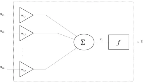
In this work, a set of neural network estimators is designed and trained in order to reproduce the behaviour of the systems under investigation, thus accomplishing the modelling and identification task. The structure of thei–th single neuron [27] is also calledperceptron. It features a MISO system where the outputyi is computed as a function f of the weighted sumviof all theni neuron inputs ui,1, . . . ,ui,ni, with the associated weightswi,1, . . . ,wi,ni. The functionf, denominatedactivation function,
represents the engine of the neuron, as shown in Figure6.
Figure 6.Thei–th neuron model comprising the neural network.
A structural categorisation of neural networks concerns the way in which their elements are connected each others [28]. In afeed–forward network, also calledmultilayer perceptron, neurons are grouped into unidirectional layers. The first of them, namely theinputlayer, is fed directly by the network inputs, then each successivehiddenlayer takes the inputs from the neurons of the previous layer and transmits the output to the neurons of the next layer, up to the lastoutputlayer, in which the final network outputs are produced. Therefore, neurons are connected from one layer to the next, but not within the same layer. The only constraint is the number of neurons in the output layer, that has to be equal to the number of actual network outputs. On the other hand,recurrent networks[29] are multilayer networks in which the output of some neurons is fed back to neurons belonging to previous layers, thus the information flow in forward as well as in backward directions allowing a dynamic memory inside the network.
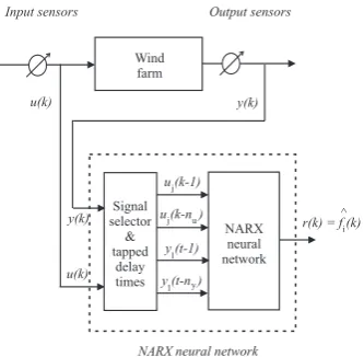
A noteworthy intermediate solution is provided by the multilayer perceptron with a tapped delay line, which is a feed–forward network whose inputs come from a delay line. This kind of network represents a suitable tool to model or predict unknown functions. In particular the open–loop NARX network belongs to this latter category as its inputs are delayed samples of the system inputs and outputs. Indeed, if properly trained, a NARX network can estimate the current (or the next) system output on the basis of the acquired past measurements of system inputs and outputs.
Generally speaking, considering a MISO system, the elaborations of the NARX neural network follow the law described by the relation of Eq. (31):
ˆ
f(k) = fnet
uh1(k−1), . . . , uh1(k−du), . . . ,uhp(k−1), . . . ,uhp(k−du) yj1(k−1), . . . , yj1(k−dy), . . . ,yjl(k−1), . . . , yjl(k−dy)
Input sensors Output sensors
Wind farm
NARX neural network
u(k) y(k)
Signal selector & tapped
delay times y(k)
u(k)
u (k-1)j
u (k-n )j u r(k) = f (k) i
NARX neural network
^
y (t-1)l
y (t-n )l y
Figure 7.The NARX neural network used as reconstructor of the general fault signal ˆfi(k).
where ˆf(k)is the estimation of the generici–th fault, whilstuhp(·)andyjl(·)are thehp–th andjl–th
measured system inputs and outputs, respectively, properly selected according to the FMEA procedure of Section3.2, with 1≤ jl≤mand 1≤hp≤m.kis the time step, whilstduanddyare the number of delays for the input and the output signals, respectively. fnetis the function realized by the network, that depends on the layer architecture, the number of neurons, their weights and their activation functions. The general fault estimation task of this NARX neural network used as fault estimator for fault diagnosis is depicted in Figure7.
The design parameters of the overall architecture are represented by its number of neurons and the connections between layers, whilst the values of the weights inside each neuron are derived from the neural network training algorithm.
A NARX neural network is a learning system requiring an initial training procedure that adjusts the weights to improve the network performance. When the network task is the estimation of a nonlinear function, the training is performed by presenting to the network a set of examples of proper behaviour, consisting of the inputsuj(·)andyl(·)(patterns), and the desired output fi(·)(target) for the relative inputs. This training phase can be implemented in two different ways:
• Incremental mode: each couple input–target generates an updating of the network weights;
• Batch mode: all inputs and targets are applied to the network before the weights are updated.
Although the latter training mode requires more memory storage capability, with respect to the former one, it is characterised by a faster convergence and produces smaller errors, thus it will be considered in the following. The training phase objective is the minimisation of a performance function E, which depends on the weight vectorw.
Generally speaking, considering a numberPof available example patterns consisting in the input–target pairs (up,tp), withp=1, . . . ,P, defining ˆypthe output generated by the network fed by up, thep–th error vector can be expressed as:
ep= [tp−yˆp] =ep,1, . . . , ep,M
T
(32)
with p = 1, . . . , PandMthe general number of outputs. Furthermore, the overall error vector ¯e collects eachep:
¯
e= [e1,1, . . . ,e1,M, . . . , eP,1, . . . , eP,M]T (33) Consequently, the performance function becomes:
E(w) = 1 P
P
∑
p=1
(ti−yˆi)2= 1 P
P
∑
p=1 M
∑
m=1
where the dependence ofEby theNparameters grouped in the vectorw= [w1, . . . , wN]Tis implicit in the generated output ˆyp=yˆp(w).
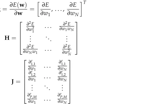
Standard numerical optimisation algorithms can be used to update the parameters, in order to minimiseE. Among these, the most commons are iterative, and make use of characteristic matrices, such as the gradientg(or the HessianH) of the performance function, or the JacobianJof the estimation error, defined as:
g= ∂E(w)
∂w =
∂E ∂w1, . . . ,
∂E ∂wN
T (35) H=
∂2E ∂w21 . . .
∂2E ∂w1wN
..
. . .. ...
∂2E ∂wNw1 . . .
∂2E ∂w2N
(36) J=
∂e1,1 ∂w1 . . .
∂e1,1 ∂wN
∂e1,2 ∂w1 . . .
∂e1,2 ∂wN
..
. . .. ...
∂eP,M ∂w1 . . .
∂eP,M ∂wN
(37)
The further iterations of these algorithms consist of the updating of the parameters and the computation of the new values of the performance function, until a stop criterion is met. The updating rules of the most common optimisation algorithms (i.e.the gradient descent, the Newton, the Gauss–Newton and the Levenberg–Marquardt algorithm) are reported in Table5.
Table 5.Updating rule parameters.
Optimisation algorithm Updating rule Gradient Descent wk+1=wk−αgk Newton wk+1=wk−H−k1gk Gauss-Newton wk+1=wk− JTkJk
−1
Jke¯k Levenberg-Marquardt wk+1=wk− JTkJk+µI−1Jke¯k
Table5summarises the parameters of the updating rules of the most common optimisation algorithms, aimed at the minimisation of the performance functionE.kis the iteration index,αis the
learning rate andµthe combination coefficient.
It can be demonstrated that the gradient descent algorithm, for a sufficiently small learning rateα
value, is asymptotically convergent: around the solutiong, the gradient is close to zero and the weights do not meaningfully change. Otherwise, the Newton and the Gauss–Newton algorithms provide a faster convergence, but they both involve the computation of the inverse of a matrix which may not be invertible, causing instability in the procedure. Moreover, the Hessian matrix entails a burdensome computational effort, as it contains the second order derivative terms.
TheLevenberg–Marquardtalgorithm, originally proposed in [30], introduces an approximation of the Hessian matrix asH≈JTJ+µI, where the first term of the sum is the Jacobian approximation (also
exploited in Gauss-Newton) and the second term, driven by the combination coefficientµ>0, ensures
the invertibility of the resulting matrix. Therefore, the Levenberg–Marquardt algorithm provides both a fast and a stable convergence and it represents a suitable tool to train a neural network. Indeed, as shown in Section5, the neural network fault estimator blocks have been trained exploiting this method.
3.4.1. Fault Diagnosis Design Procedure
The complete design flow relying on both fuzzy systems and neural networks used as fault estimators for fault diagnosis is summarised in Figure8.
Figure 8.Fault diagnosis design procedure block diagram.
Finally, note that the design flow sketched in Figure8assumes that only single faults affect the process under diagnosis.
4. Model–Based Fault Diagnosis Method
This section recalls the purely nonlinear fault diagnosis scheme that represents a model–based approach mainly used for comparison purpose, as summarised in Section5. In particular, this method is based on analytical physical law modelling and partially on parameter estimation of some coefficients describing this mathematical relations.
The proposed fault diagnosis scheme consists of three phases. The first step regards the estimation of the nonlinear disturbance distribution functions, which are required for the design of the nonlinear adaptive filter for fault estimation. The fault reconstruction is thus exploited for fault diagnosis purposes of the measured signals.
already investigated in [11] but applied to a single wind turbine. It will be used here and applied to the wind turbine models of the wind farm. The second disturbance effect is due to the interactions among the wind turbines of the wind farm, and represented by the wind wakes [2].
Solutions dealing with the first disturbance term were based on the estimation of both the wind turbine power coefficientCpvalues and the wind speedvw(t). It is worth noting that, regarding the wind wakes, a novel strategy based on a nonlinear design scheme is proposed here. In particular, as for the decoupling of the wind speedvw(t)addressed in [11], this approach required the analytical knowledge of the nonlinear disturbance distribution relation of the unknown inputs represented by the wake effects. In more detail, as shown in [11], the power coefficientCp–map appearing in the wind turbine aerodynamic models of the wind farm was estimated by means of a two–dimensional polynomial representation, which was a function of the tip–speed ratioλand the blade pitch anglesβ
[32].
Once the disturbance description has been obtained in analytical form, the second stage of the fault diagnosis system design is based on the development of the nonlinear fault diagnosis filters. Their structure is obtained by exploiting a disturbance decoupling scheme belonging to the NLGA framework [33]. A coordinate transformation, highlighting a subsystem affected by the fault and decoupled by the disturbances, represents the starting point to design adaptive filters for fault estimation. It is worth observing that, by means of this NLGA approach, the fault estimate is decoupled from the disturbance d, which in this work are represented by the wake effects of the wind turbines affecting thei–th wind turbine of the wind farm.
Therefore, the proposed approach is applied to the general nonlinear model in the form of Eq. (38):
(
˙
x = n(x) +g(x)c+`(x)f +pd(x)d
y = h(x) (38)
where the state vectorx∈ X (an open subset ofR`n),c(t)∈R`cis the control input vector, f(t)∈Ris the fault,d(t)∈R`d is the disturbance vector, andy∈R`m is the output vector.n(x),`(x), the columns
ofg(x), andpd(x)are smooth vector fields, withh(x)a smooth map.
The development of the NLGA strategy for the design of the estimator for the fault f with the decoupling of the disturbancedis based on the procedure presented in [34]. It was shown that the considered NLGA scheme extended to the fault diagnosis problem is based on a coordinate change in the state space and in the output space, such that, by using the new (local) state and output coordinates (x¯, ¯y), the system of Eq. (38) is transformed into [34]:
˙¯
x1 = n1(x1¯ , ¯x2) +g1(x1¯ , ¯x2)c+`1(x1¯ , ¯x2, ¯x3)f ˙¯
x2 = n2(x¯1, ¯x2, ¯x3) +g2(x¯1, ¯x2, ¯x3)c+ +`2(x¯1, ¯x2, ¯x3)f +p2(x¯1, ¯x2, ¯x3)d ˙¯
x3 = n3(x1¯ , ¯x2, ¯x3) +g3(x1¯ , ¯x2, ¯x3)c+ +`3(x1¯ , ¯x2, ¯x3)f +p3(x1¯ , ¯x2, ¯x3)d ¯
y1 = h(x¯1) ¯
y2 = x2¯
(39)
with`1(x1¯ , ¯x2, ¯x3)not identically zero. As remarked in [34], this procedure yields to the observable ¯x1 subsystem of Eq. (39) that, if it exists, is affected by the faults f, and not affected by disturbancesd.
This transformation can be applied to the system of Eq. (38), if and only if some fault detectability conditions are satisfied [34]. The system of Eq. (38) in the new reference frame is decomposed into 3 subsystems of Eqs. (39), where the first one (the so–called ¯x1–subsystem) is always decoupled from the disturbancesdand affected by the faultsf, described in the form of Eq. (40):
(
˙¯
x1 = n1(x1¯ , ¯y2) +g1(x1¯ , ¯y2)c+`1(x1¯ , ¯y2, ¯x3)f ¯
y1 = h(x¯1)
where, as the state ¯x2in Eq. (39) is assumed to be measured, the variable ¯x2in Eq. (40) is considered as independent input, and denoted with ¯y2.
The proposed NLGA adaptive filter is based on the least–squares algorithm with forgetting factor described by the adaptation law of Eq. (41):
(
˙
P =βP− N12P2M˘21, P(0) =P0>0 ˙ˆ
f =PeM˘1, fˆ(0) =0
(41)
with Eq. (42) representing the output estimation, and the corresponding normalised estimation error:
(
ˆ¯
y1s = M1˘ fˆ+M2˘ +λy1˘¯ s
e = N12 (y¯1s−yˆ¯1s)
(42)
where all the involved variables of the adaptive filter are scalar. In particular,λ>0 is a parameter
related to the bandwidth of the filter, β ≥ 0 is the forgetting factor, and N2 = 1+M˘21 is the
normalisation factor of the least–squares algorithm. Moreover, the proposed adaptive filter adopts the signals ˘M1, ˘M2, ˘¯y1swhich are obtained by means of a low–pass filtering of the signalsM1,M2, ¯y1sas follows:
˙˘
M1 =−λM1˘ +M1, M1˘ (0) =0 ˙˘
M2 =−λM2˘ +M2, M2˘ (0) =0 ˙˘¯
y1s =−λy˘¯1s+y¯1s, y˘¯1s(0) =0
(43)
The considered adaptive filter is described by the systems of Eqs. (41), (42), and (43). It is worth noting that in [34] it was showed that this adaptive filter provides an estimation ˆf(t)that asymptotically converges to the magnitude of the actual fault f.
This completes the design of the fault diagnosis methodology based on NLGA adaptive filters, whose results will be shown in Section5.
5. Simulation Results
The following simulations refers to the wind farm benchmark model when the fault diagnosis schemes based on the fuzzy and neural network fault estimators are designed.
The mean wind sequence driving all the simulations covers the most common operative range from 5 m/s up to 15 m/s, with a peak value of about 23 m/s. The wind and wake submodel described in Section2processes this sequence in order to generate the actual wind speed signal for all the turbines of the wind farm and for both the measurement musts associated with the two wind scenarios provided by the benchmark model, as shown in Section2, also taking into account the disturbances and the interaction among turbines. Figure9depicts the leading wind sequence.
The available data consist of 440000 samples of input–output measurements, acquired with a sampling rate of 100 Hz.
The 3 proposed faults described in Section2affect different wind turbines at different times, by influencing the measured variablesu(k)andy(k), and in particular the signalsβi,ωg,i,Pg,irelated with thei–th wind turbine of the wind farm. These faults are difficult to detect at wind turbine level. However, they can be more easily detected at wind farm level, by comparing the performance of different wind turbines. Table6shows the affected turbines per fault, together with the occurrence time.
These faults are simulated for the 3 cases of Table1and under the assumptions described in Section2.3.
5.1. Fuzzy Estimator Results
Figure 9.The mean wind speed sequence driving the simulations of the wind farm.
Table 6.Faulty turbines and activation times.
Fault Affected Turbine Time (s)
1 7 1000-1100
2 3000-3100
2 1 1300-1400
5 3300-3400
3 6 1600-1700
8 3600-3700
FMEA recalled in Section3.1. The TS models exploit Gaussian membership functions. Afterwards, the fault estimators are organised into a dedicated observer scheme of Section3.1that allows for the isolation of the 3 faults affecting the wind farm benchmark model described in Section2.3.
Firstly, the capabilities of these 3 fuzzy fault estimators are evaluated in terms of RMSE, defined as the per cent difference between the measurements and the estimation, computed in fault free conditions. This index can be considered as the measure of the percentage of the data not correctly reconstructed by the estimator. As highlighted in Table7, although this index increases when computed on data which are not used in the estimation phase (i.e.validation and test data sets), however, the percentage is always smaller than 5%, thus featuring a good modelling capability.
Table 7.RMSE of the fuzzy fault estimators.
Data Set RMSE(%)
Fault 1 Estimator Fault 2 Estimator Fault 3 Estimator
Estimation 0.0090 0.0087 0.0092
Validation 0.0103 0.0101 0.0105
Test 0.0108 0.0103 0.0109
Then, the detection of the 3 faults is achieved by means of the residualsri(k) = fˆi(k)generated by the fault estimators, after the proper tuning of the threshold parameterδ. In particular, Figure10
highlights the residualr1(k)relative to the fault 1 estimator, whose value is bounded by the thresholds when the fault is not active, while it is significantly over the threshold when the fault occurs on the two different turbines. Similar results are achieved by the fault 2 and 3 estimators, whose residuals r2(k)andr3(k)are depicted in Figures11and12, respectively.
5.2. Neural Network Estimator Results
0 1000 2000 3000 4000 0
0.2 0.4 0.6 0.8 1
Time (s)
Estimation of the fault 1:
f (k)
^
1r (k)
1[]
Figure 10.Fault 1 estimator residualr1(k)(continuous lines) and its threshold level (dotted line).
Time (s)
r (k)
2Estimation of the fault 2:
f (k)
^
2
0 1000 2000 3000 4000
0 0.1 0.2 0.3
[°]
Figure 11.Fault 2 estimator residualr2(k)(continuous lines) and its threshold level (dotted line).
the FMEA procedure of Section3.2and the considered fault cases. The selected architecture of the networks involves two layers, namely the hidden layer and the output layer. The number of neurons in the hidden layer has been fixed tonh = 16. A number ofdu = dy = 5 has been chosen for the input–output delays. Similarly to the fuzzy models, the neural networks modelling capabilities have been tested in terms of RMSE and the results are reported in Table8in fault–free conditions for three different data sets (training, validation and test).
Table 8.Neural network performance in terms of RMSE %.
Fault Estimator 1 2 3
RMSE % (training set) 0.0089 0.0091 0.0092 RMSE % (validation set) 0.0091 0.0093 0.0095 RMSE % (validation set) 0.0106 0.0104 0.0123
Time (s)
r (k)
3Estimation of the fault 3:
f (k)
^
3[]
0 1000 2000 3000 4000
0 20 40 60 80 100
Figure 12.Fault 3 estimator residualr3(k)(continuous lines) and its threshold level (dotted line).
Table 9. The optimal values of the parameterδused for fault diagnosis purposes by the designed
residual generators.
Residualri(k) = fˆi(k) δfor the fuzzy estimators δfor the neural network estimators
1 2.15 2.34
2 2.23 2.45
3 2.34 2.89
5.3. Fault Diagnosis NLGA Simulations
This section describes the design and the simulations of the NLGA adaptive filters applied to the wind park benchmark. In particular, the results achieved from the estimation of the disturbance terms appearing in Eq. (38) are firstly presented. Once the disturbance decoupling has been achieved, the performances of the NLGA fault estimators are reported.
In more detail, thei–th Cp–map entering into the aerodynamic model of each of the 9 wind turbines of the wind farm described in Section2has been approximated by using the two–dimensional polynomial in the form of Eq. (44):
ˆ
Cp(λi,βi) =0.010λ2i +0.0003λ3i βi−0.0013λ3i (44)
for thei–th turbine of the wind park. More details they can be found in [32]. By following the same procedure, the second disturbance term representing thepd(x)function in Eq. (38) is described by the polynomial ˆCpi representing the wind wake from thej–th turbine of the park affecting thei–th turbine: pd(x) =0.0027λ2j βj−0.0011λ2j (45)
withi6=j. In general, note that the expression of both the ˆCpi–map and the disturbance termpd(x)in Eq. (45) depend on thei–th wind turbine of the wind farm.
case is that the model–reality mismatch is varying more slowly that the disturbance signals, such asd. Another important point regards the fact that thepd(x)estimation aims at describing the structure of the uncertainty, which should not depend on the wind size uncertainty. Only the so–called ’directions’ of the disturbance represent the important effect for disturbance decoupling,i.e.thepd(x)term, and not the ’amplitude’ of the uncertainty,i.e.the size of the disturbanced.
The designed NLGA adaptive filters of Eqs. (41), (42), and (43) provide the estimate the magnitude of the different faults acting on the the wind farm benchmark, as shown in Section4. With reference to the overall input–affine model of the wind farm described in Section2, the following terms can be determined:
n(x) =
"
−ρA
2J 0.0010R3x21−1J x2
−pgenx2
#
(46)
g(x) =
"
0 ρ2AJ 0.0003R3x22
pgen 0
#
(47)
and:
`(x) =
"
0 ρ2AJ 0.0003R3x21 0 0.0001
#
(48)
with reference to thei–th turbine, with the understanding that the subscriptiis dropped. Moreover, pd(x)is defined as:
pd(x) =
" ρA
2J 0.0010R2x1 0.0011 0.0002 ρA
2J 0.0027x2
#
(49)
In the case of the model of Eq. (38), and recalling Eqs. (49), (48), and (47), it results that:
S0=P¯=cl(pd(x))≡pd(x) (50) If ker{dh} = ∅, it follows thatΣP∗ = P¯ as ¯S0∩ker{dh} = ∅. On the other hand, it is necessary
to compute the expression ΣP
∗
⊥
= (P¯)⊥. However, it is worth noting that, for the case under investigation, the determination of the codistribution ΣP∗
⊥
= (P¯)⊥is enhanced due to the structure of Eq. (50).
Finally, as an example, the design of the NLGA adaptive filter for the reconstruction of the fault case 2 is based on the expression of Eq. (51):
˙¯
y1s =M1·f +M2 (51)
where:
(
M1 = 0.8x21−0.036x1
M2 = 1.02x22+15.7x2−0.3x31+0.77x21 (52) The design of the NLGA adaptive filters for the reconstruction of the faults for the cases 1 and 3 is based on a different selection of the vector of Eq. (48), which leads to other expressions for the filter of Eq. (51). As an example, for the fault case 2 described in Section2.3, the nonlinear filter for the reconstruction of f2decoupled from the disturbancedrepresenting the effect of both the wind vw(t)and the wakevw,msignals has the form of Eq. (41). After a suitable choice of the parameters in Eqs. (41), (42), and (43) the nonlinear filter provided an accurate estimate ˆf2(k)of the fault size, with minimal detection delay.
Finally, also the model capabilities of the 3 NLGA estimators with disturbance decoupling are evaluated in terms of RMSE %, as summarised in Table10, thus demonstrating the superiority of the model–based approach with respect to the data–driven methods.
Table 10.RMSE of the NLGA fault estimator with disturbance decoupling.
Fault Case Fault 1 Estimator Fault 2 Estimator Fault 3 Estimator
RMSE(%) 0.0007 0.0008 0.0009
5.4. Validation and Comparative Analysis
The evaluation of the performances of the considered fault diagnosis strategies is based on the computation of the following indices:
• False Alarm Rate (FAR): the ratio between the number of wrongly detected faults and the number of simulated faults;
• Missed Fault Rate(MFR): the ratio between the total number of missed fault (detection/isolation) and the number of simulated faults;
• True Fault diagnosis Rate(TFR): the ratio between the number of correctly detected/isolated faults and the number of simulated faults (complementary to MFR);
• Mean Fault diagnosis Delay(MFD): the delay time between the fault occurrence and the fault detection/isolation.
A proper Monte–Carlo analysis has been performed in order to compute these indices and to test the robustness of the considered fault diagnosis schemes. Indeed, the Monte–Carlo tool is useful at these stage, as the efficacy of the diagnosis depends on both the model approximation capabilities and the measurements errors.
In particular, extensive simulations based on a set of 10000 Monte–Carlo runs has been executed, during which realistic wind turbine uncertainties have been considered. Some meaningful variables have been modelled as Gaussian white stochastic processes with nominal values and standard deviations corresponding to realistic error values summarised in Table11.
Table 11.Monte–Carlo analysis parameter variations.
Parameter Nominal Value Error Value
ρ 1.225Kg/m3 ±20%
J 7.794×10⁶Kg/m3 ±30%
Cp Cp0 ±50%
The comparative analysis results are reported in Table12. In particular, the different approaches to the fault diagnosis of the wind farm benchmark model,i.e.the fuzzy, the neural network and the NLGA adaptive filter fault estimators, are shown.
Table 12.Comparison of the fault diagnosis results with the different fault diagnosis strategies.
Fault Case Index Fuzzy Systems Neural Networks NLGA Filters
1 FAR 0.0010 0.0010 0.0006
MFR 0.0010 0.0010 0.0007
TFR 0.9990 0.9990 0.9994
MFD (s) 0.02 0.01 0.007
2 FAR 0.0010 0.2280 0.0004
MFR 0.0030 0.0010 0.0005
TFR 0.9970 0.9990 0.9996
MFD (s) 0.08 0.08 0.008
3 FAR 0.0030 0.0010 0.0005
MFR 0.0080 0.0010 0.0006
TFR 0.9920 0.9990 0.9995
MFD (s) 0.02 0.01 0.006
a noteworthy performance level considering the MFD. Also the FAR and MFR are quite low, and in particularly neural networks present very low values of MFR for all the considered faults. However, for both fuzzy and neural networks fault diagnosis design, optimisation stages are required, for example for the selection of the optimal thresholds. On the other hand, the NLGA adaptive estimators definitely show the best results, with respect to the MFD index and the least TFR, with respect to the other fault diagnosis methodologies. However, the design complexity is much higher than the other approaches, and in some cases the analytic solution cannot be achieved.
Finally, the achieved results also lead to further considerations: the proper choice of the design parameters can lead to the least FAR and MFR, with very high TDR, and minimal MFD. Moreover, the Monte–Carlo analysis validates the robustness and the estimation convergence properties of the proposed fault diagnosis schemes, with respect to error, noise and uncertainty.
6. Conclusion
The paper proposed different solutions to the problem of earlier fault detection and diagnosis with application to a wind farm benchmark. The proposed design was based on fault estimators relying on data–driven approaches, as they represented effective tools for coping with a poor analytical knowledge of the system dynamics, together with noise and disturbances. In particular, the data–driven proposed solutions exploited fuzzy systems and neural networks used to describe the strongly nonlinear relationships between the wind farm measurements and its faults. The chosen fuzzy prototype and network architecture belongs to the nonlinear autoregressive with exogenous input topology, as it can represent a dynamic evolution of the system along time. The developed fault diagnosis schemes were tested by means of a high–fidelity benchmark model, that simulated the normal and the faulty behaviour of a wind farm system. The achieved performances were compared with those of a different fault diagnosis strategy, based on analytical modelling of the physical laws, and relying on a nonlinear disturbance decoupling methodology. Moreover, a Monte–Carlo analysis served to analyse the robustness and reliability features of the proposed solutions against typical parameter uncertainties and disturbances. Further works will address the analysis of the performance of the developed fault diagnosis strategies when used for active fault tolerant control schemes, and possibly with application to real wind turbine systems.
Sample Availability:The software simulation codes for the proposed control strategies and the simulated wind farm benchmark are available from the authors in the MATLAB and Simulink environments.
Acknowledgments:The research works have been supported by the FAR2016 local fund from the University of Ferrara. On the other hand, the costs to publish in open access have been covered by the FIR2016 local fund from the University of Ferrara.
Author Contributions: Saverio Farsoni conceived and designed the simulations. Silvio Simani analysed the methodologies, the achieved results, and together with Paolo Castaldi, wrote the paper.
Conflicts of Interest:The authors declare no conflict of interest.
References
1. Odgaard, P.; Patton, R. FDI/FTC wind turbine benchmark modelling. Workshop on Sustainable Control of Offshore Wind Turbines; Patton, RJ, Ed, 2012.
2. Odgaard, P.F.; Stoustrup, J. Fault tolerant wind farm control. A benchmark model. Control Applications (CCA), 2013 IEEE International Conference on. IEEE, 2013, pp. 412–417.
3. Odgaard, P.F.; Stoustrup, J. A benchmark evaluation of fault tolerant wind turbine control concepts. Control Systems Technology, IEEE Transactions on2015,23, 1221–1228.
4. Chen, W.; Ding, S.X.; Sari, A.; Naik, A.; Khan, A.Q.; Yin, S. Observer-based FDI schemes for wind turbine benchmark. Proceedings of IFAC world congress, 2011, Vol. 18, pp. 7073–7078.
5. Gong, X.; Qiao, W. Bearing fault diagnosis for direct-drive wind turbines via current-demodulated signals.
6. Parker, M.A.; Ng, C.; Ran, L. Fault-tolerant control for a modular generator–converter scheme for direct-drive wind turbines.Industrial Electronics, IEEE Transactions on2011,58, 305–315.
7. Odgaard, P.F.; Stoustrup, J. Results of a wind turbine FDI competition. 8th IFAC symposium on fault detection, supervision and safety of technical processes, 2012, pp. 102–107.
8. Odgaaard, P.F.; Shafiei, S.E. Evaluation of Wind Farm Controller based Fault Detection and Isolation.
IFAC-PapersOnLine2015,48, 1084–1089.
9. De Persis, C.; Isidori, A. A geometric approach to nonlinear fault detection and isolation. Automatic Control, IEEE Transactions on2001,46, 853–865.
10. Castaldi, P.; Mimmo, N.; Simani, S. Differential Geometry Based Active Fault Tolerant Control for Aircraft.
Control Engineering Practice2014,32, 227–235. Invited Paper. DOI:10.1016/j.conengprac.2013.12.011. 11. Simani, S.; Castaldi, P. Active actuator fault-tolerant control of a wind turbine benchmark model.International
Journal of Robust and Nonlinear Control2014,24, 1283–1303. 12. Jensen, N.O.A note on wind generator interaction; 1983.
13. Johnson, K.E.; Pao, L.Y.; Balas, M.J.; Fingersh, L.J. Control of variable-speed wind turbines: standard and adaptive techniques for maximizing energy capture. Control Systems, IEEE2006,26, 70–81.
14. Fantuzzi, C.; Simani, S.; Beghelli, S.; Rovatti, R. Identification of piecewise affine models in noisy environment.
International Journal of Control2002,75, 1472–1485.
15. Chen, J.; Patton, R.J.Robust model-based fault diagnosis for dynamic systems; Vol. 3, Springer Science & Business Media, 2012.
16. Stamatis, D.H.Failure mode and effect analysis: FMEA from theory to execution; ASQ Quality Press, 2003. 17. Takagi, T.; Sugeno, M. Fuzzy identification of systems and its applications to modeling and control.Systems,
Man and Cybernetics, IEEE Transactions on1985, pp. 116–132.
18. Babuška, R.Fuzzy modeling for control; Vol. 12, Springer Science & Business Media, 2012.
19. Fantuzzi, C.; Rovatti, R. On the approximation capabilities of the homogeneous Takagi-Sugeno model. Fuzzy Systems, 1996., Proceedings of the Fifth IEEE International Conference on. IEEE, 1996, Vol. 2, pp. 1067–1072.
20. Rovatti, R. Takagi-Sugeno models as approximators in sobolev norms: the siso case. Fuzzy Systems, 1996., Proceedings of the Fifth IEEE International Conference on. IEEE, 1996, Vol. 2, pp. 1060–1066.
21. Jain, A.K.; Murty, M.N.; Flynn, P.J. Data clustering: a review. ACM computing surveys (CSUR)1999,
31, 264–323.
22. Jun, W.; Shitong, W.; Chung, F.l. Positive and negative fuzzy rule system, extreme learning machine and image classification. International Journal of Machine Learning and Cybernetics2011,2, 261–271.
23. Graaff, A.J.; Engelbrecht, A.P. Clustering data in stationary environments with a local network neighborhood artificial immune system.International Journal of Machine Learning and Cybernetics2012,3, 1–26.
24. Bezdek, J.C.Pattern recognition with fuzzy objective function algorithms; Springer Science & Business Media, 2013.
25. Simani, S.; Fantuzzi, C.; Rovatti, R.; Beghelli, S. Parameter identification for piecewise-affine fuzzy models in noisy environment.International Journal of Approximate Reasoning1999,22, 149–167.
26. Beghelli, S.; Guidorzi, R.P.; Soverini, U. The Frisch scheme in dynamic system identification. Automatica
1990,26, 171–176.
27. Haykin, S.S.; Haykin, S.S.; Haykin, S.S.; Haykin, S.S.Neural networks and learning machines; Vol. 3, Pearson Education Upper Saddle River, 2009.
28. Liu, G.P.Nonlinear identification and control: a neural network approach; Springer Science & Business Media, 2012.
29. Medsker, L.; Jain, L.C.Recurrent neural networks: design and applications; CRC press, 1999.
30. Marquardt, D.W. An algorithm for least-squares estimation of nonlinear parameters. Journal of the society for Industrial and Applied Mathematics1963,11, 431–441.
31. Hagan, M.T.; Menhaj, M.B. Training feedforward networks with the Marquardt algorithm. Neural Networks, IEEE Transactions on1994,5, 989–993.
32. Simani, S.; Castaldi, P. Estimation of the power coefficient map for a wind turbine system. Proceedings of the 9th European Workshop on Advanced Control and Diagnosis (ACD’11), 2011, number paper 13, pp. 1–7. 33. De Persis, C.; Isidori, A. On the observability codistributions of a nonlinear system.Systems & control letters