An EOQ Model for Weibull Deteriorating Items with Linear Demand and Partial Backlogging in Fuzzy Environment

Available Online atwww.ijcsmc.com

International Journal of Computer Science and Mobile Computing

A Monthly Journal of Computer Science and Information Technology

ISSN 2320–088X

IJCSMC, Vol. 4, Issue. 12, December 2015, pg.242 – 254

An EOQ Model for Weibull Deteriorating

Items with Linear Demand and Partial

Backlogging in Fuzzy Environment

J.Sujatha

1

, P.Parvathi

2 1

Asst. Professor, Dept. of Mathematics, Quaid-E-Millath Govt. College for Women(A), Chennai, India 2

Head & Assoct.Professor, Dept. of Mathematics, Quaid-E-Millath Govt. College for Women(A),Chennai, India

Abstract --- In this paper, we developed an EOQ model for Weibull deteriorating items with linear demand rate in fuzzy environment. Shortages are allowed and partially backlogged. Holding cost, deterioration cost, ordering cost, shortage cost and opportunity cost are assumed as a triangular fuzzy numbers. The purpose of this paper is to minimize the total cost function in fuzzy environment. Graded mean representation, signed distance and centroid methods are used to defuzzify the total cost function and the results obtained by these methods are compared with the help of a numerical example. Sensitivity analysis is also carried out to detect the most sensitive parameters of the system.

Keywords--- EOQ model, Two parameter Weibull deteriorating items, Shortages, Triangular fuzzy number, Graded mean representation method, Signed distance method, Centroid method.

I. INTRODUCTION

Bhunia and Maiti (1998) [15] developed an a two warehouse inventory model for deteriorating items with a linear demand and shortages. Goswami and Chandhuri (1991) [16] developed an EOQ model for deteriorating items with a linear trend in demand.

In conventional inventory models, uncertainties are treated as randomness and are being handled by applying the probability theory. However, in certain situations uncertainties are due to fuzziness, and such cases are dilated in the fuzzy set theory which was demonstrated by Zadeh in [17]. Kauffmann and Gupta [18] provided an introduction to fuzzy arithmetic operation and Zimmermann [19] discussed the concept of the fuzzy set theory and its applications. Considering the fuzzy set theory in inventory modelling renders an authenticity to the model formulated since fuzziness is the closest possible approach to reality. As reality is imprecise and can only be approximated to a certain extent, same way, fuzzy theory helps one to incorporate uncertainties in the formulation of the model, thus bringing it closer to reality. Park [20] applied the fuzzy set concepts to EOQ formula by representing the inventory carrying cost with a fuzzy number and solved the economic order quantity model using fuzzy number operations based on the extension principle. Vujosevic et al. [21] used trapezoidal fuzzy number to fuzzify the order cost in the total cost of the inventory model without backorder, and got fuzzy total cost. Yao and Lee [22] introduced a backorder inventory model with fuzzy order quantity as triangular and trapezoidal fuzzy numbers and shortage cost as a crisp parameter.

Chang [23] discussed the fuzzy production inventory model for fuzzify the product quantity as triangular fuzzy number. Yao and Chiang [24] considered the total cost of inventory without backorder. They fuzzified the total demand and cost of storing one unit per day into triangular fuzzy numbers and defuzzify by the centroid and the signed distance methods. Gani and Maheswari[25] developed an EOQ model with imperfect quality items with shortages where defective rate, demand, holding cost, ordering cost and shortage cost are taken as triangular fuzzy numbers. Graded mean integration method is used for defuzzification of the total profit. Uthayakumar and Valliathal [26] developed an economic production model for Weibull deteriorating items over an infinite horizon under fuzzy environment and considered some cost component as triangular fuzzy numbers and using the signed distance method to defuzzify the cost function.

In this paper, an inventory model for Weibull deteriorating items and linear demand with shortages is considered where , ordering cost, holding cost, deterioration rate, , shortage cost and opportunity cost are assumed as a triangular fuzzy numbers. For defuzzification of the total cost function, Graded Mean Representation, Signed distance and Centroid methods are used. By comparing the results obtained by these methods, we get the better one as an estimate of the total cost in the fuzzy sense.

II. FUZZY PRELIMINARIES

In order to treat fuzzy inventory model by using graded mean representation, signed distance and centroid to defuzzify , we need the following definitions.

Definition 2.1 A fuzzy set

a

~

on

R



(



,



)

is called a fuzzy point if its membership function is



















a

x

a

x

x

a

,

0

,

1

)

(

~



--- (1)

where the point a is called the support of fuzzy set

a

~

Definition 2.2 A fuzzy set



a

_

,

b

_



where

0







1

and a < b defined on R, is called a level of a fuzzy interval if its membership function is

_{ }



















otherwise

b

x

a

x

b a

,

0

,

)

(

,







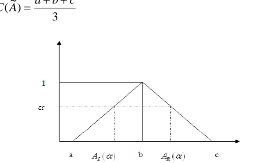
Definition 2.3 A fuzzy number A~(a,b,c) where a < b < c and defined on R, is called a triangular fuzzy number if its membership function is

        

   

   



otherwise c x b b c

x c

b x a a b

a x

A

, 0

, ,



--- (3)

When

a



b



c

,

we have fuzzy point

(

c

,

c

,

c

)



~

c

The family of all triangular fuzzy numbers on R is denoted as

F

_N







a

,

b

,

c



a



b



c



a

,

b

,

c



R



.

The



-cut of A~(a,b,c)F_N,0 1, is A(



)



A_L(



),A_R(



)



WhereA_L(



)a(ba)



and





)

(

)

(

c

c

b

A

_R







are the left and right endpoints of A (



).

Definition 2.4 If

A

~



(

a

,

b

,

c

)

is a triangular fuzzy number then the graded mean integration representation of

A

~

is defined as







_







_





 

A A

w w

hdh

dh

h

R

h

L

h

A

P

0 0

1 1

2

)

(

)

(

)

~

(

With

0



h



w

A and

o



w

A



1





6

4

)

(

)

(

2

1

)

~

(

₁

0 1

0

a

b

c

hdh

dh

a

c

h

c

a

b

h

a

h

A

P























--- (4)

Definition 2.5 If

A

~



(

a

,

b

,

c

)

is a triangular fuzzy then the signed distance of

A

~

is defined as

 













1

0

0

~

,

)

(

,

)

(

0

~

,

~









_R

L

A

A

d

A

d





a



2

b



c



4

1

--- (5)

Definition 2.6 The centroid method on the triangular fuzzy number

A

~



(

a

,

b

,

c

)

is defined as

3

)

~

(

A

a

b

c

C







--- (6)

III. NOTATIONS AND ASSUMPTIONS The proposed inventory model having following notations and assumptions: 3.1 Notations

I(t) : the inventory level at time t.

W : the maximum inventory level for each ordering cycle.

IB : the maximum amount of demand backlogged for each ordering cycle. Q : the economic order quantity for each ordering cycle.

T : length of each ordering cycle. 1

C

: deterioration cost , $/per unit. 2

C

: shortage Cost, $/per unit /per unit time. 3

C

_{: opportunity cost,$/ per unit /per unit time.}

h(t) : holding cost , $/per unit/ per unit time. A : ordering cost of inventory, $/ per order

1

~

C

: fuzzy deterioration cost, $/per unit. 2

~

C

: fuzzy shortage cost, $/per unit/ per unit time. 3

~

C

_{: fuzzy opportunity cost,$/ per unit /per unit time.}

h

~

: fuzzy holding cost, $/per unit/ per unit time.

A

~

_{: fuzzy ordering cost of inventory, $/ per order.}

)

,

(

T

₁

T

TC

: total inventory cost per unit time.

) , ( ~

1 T

T C

T : total fuzzy inventory cost per unit time.

)

,

(

T

1

T

TC

dG : defuzzify value of ( , )

~

1 T T C

T by applying Graded mean integration method

)

,

(

T

₁

T

TC

_dS

: defuzzify value of ( , ) ~

1 T

T C

T by applying Signed distance method

)

,

(

T

1

T

TC

dC : defuzzify value of ( , )

~

1 T

T C

T by applying Centroid method 3.2 Assumptions:

(i) The inventory system involves only one item and the planning horizon is infinite. (ii) Replenishment occurs instantaneously at an infinite rate.

(iii) The demand rate ,

  

  



0 ) ( ,

0 ) ( ,

) (

0 whenI t

D

t whenI bt

a t D

where a >0 , b > 0 and a is initial demand.

(iv) The deterioration of time as follows by Weibull parameters (two) distribution

(

)

,

1





_





t

t

where

0







1

is the scale parameter and  0 is the shape parameter.

(v) During the shortage period, the backlogging rate is variable and is dependent on the length of the waiting time for the next replenishment. The longer the waiting time is, the smaller the backlogging rate would be. Hence, the proportion of customers who would like to accept backlogging at time t is decreasing with the waiting time

T



t

waiting for the next replenishment. To take care of this situation we have defined the backlogging rate to be

) ( 1

1

t T 

 when

IV. MATHEMATICAL MODEL 4.1 Crisp Model:

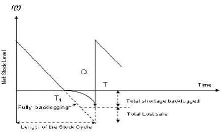
Figure 2: Graphical representation of the inventory system

We consider the deteriorating inventory model with linear demand. Replenishment occurs at time t= 0 when the inventory level attains its maximum W . From t = 0 to

T

₁ , the inventory level reduces due to demand and deterioration. At time

T

₁ the inventory level achieves zero, then shortage is allowed to occur during the time interval



T1,T



and all of the demand during shortage period



T

1

,

T



is partially backlogged.

As the inventory level reduces due to demand rate as well as deterioration during the inventory interval



T1,T



,

the differential equation representing the inventory status is governed by

;

0



t



T

₁

Where



(

t

)





t

1 and

D

(

t

)



a



bt

;

0



t



T

₁ --- (7)

During the shortage interval [T1, T] , the demand at time t is partially backlogged at the fraction )

( 1

1 t T 

 . Therefore, the differential equation governing the amount of demand backlogged is

;

T

₁



t



T

--- (8) where

D

(

t

)



D

₀ with the boundary condition

I

(

T

₁

)



0

and

I

(

0

)



W

. The solution of equation (7) and (8) is given by





















































































 

 

 

  



)

(

2

)

(

1

)

(

2

)

(

2

)

(

1

)

(

)

(

2

)

(

2 2 2 1 2

1 2 1 1 2 2

2 1 1

1

2 2 1 1

1 1 2

2 1 1

  

   

 



  























t

t

T

b

t

t

T

a

t

t

T

b

t

t

T

a

t

T

b

t

T

a

t

T

b

t

T

a

t

I

;

0



t



T

1

--- (9) )

( ) ( )

( 1

bt a t

I t dt

t

dI _

_

 _{ }

) ( 1 )

( 0

t T D dt

t dI

   



) ( )

( ) ( ) (

t D t

I t dt

t

( ) log



1 ( )



log



1 ( 1)



0

0

T T D

t T D

t

I     











;T1 t T --- (10)

Maximum amount of demand backlogged per cycle is obtained by putting in t = T in Equation (10). Therefore,



1 ( )



log )

( 1

0

T T D

T I

IB  







--- (11)

Maximum inventory level for each cycle is obtained by putting the boundary condition

I

(

0

)



W

in equation (9). Therefore,

2 1

2

2 1 1

1 2

1

1  _  _

  









 

T b T

a T b aT

W --- (12) Hence, the economic order quantity per cycle is



1 ( )



log 2

1

2 1

0 2 1 1

1 2

1

1 T T

D T

b T

a T b aT IB W

Q   

    

 

  













 

--- (13)

The total cost per cycle consists of following cost components (i) Inventory holding cost over the cycle is given by

HC=



1

0

)

(

)

(

T

dt

t

I

t

h



     

      

 

  



 

  

 

 _{ }

 

) 3 2 )( 1 ( ) 2 2 )( 1 (

) 3 )( 1 ( ) 2 )( 1 ( 3 2

3 2 1 2 2

2 1 2

3 1 2

1 3

1 2 1

























 

 

T b T

a

T b T

a bT

aT h

--- (14)

(ii) Deterioration cost over the cycle is given by

    

  





_

1

0

1 ( )

T

dt t D W

C DC





















 

2

1

2 1 1

1

1

_







 

T

b

T

a

C

--- (15)

(iii) Shortage cost over the cycle is given by







T

T

dt

t

I

C

SC

1

)

(

2

C D





_{T t}





_{T T}





_dt

T

T



     



1

) ( 1 log ) ( 1

log 1

0

2

























_

_

_



1

1

₂

log

1

(

₁

)

0

2

T

T

T

T

D

C





(iv) The opportunity cost due to lost sales per cycle is

_dt

t

T

D

C

OC

T

T



































1

1

(

)

1

1

0 3

_





      _{   }

C₃D₀ T T₁ 1log1



(T t)



--- (17)

(v) Ordering cost per cycle

OC = A --- (18)

Total cost of the system per unit time is given by



HC DC SC OC A



T T T

TC( 1, ) 1    









                             _{   }         _{  }                                      T A t T T T T D C T T T T T D C T b T a T C T b T a T b T a bT aT T h T T TC ) ( 1 log 1 ) ( 1 log 1 2 1 ) 3 2 )( 1 ( ) 2 2 )( 1 ( ) 3 )( 1 ( ) 2 )( 1 ( 3 2 ) , ( 1 0 3 1 2 1 0 2 2 1 1 1 1 3 2 1 2 2 2 1 2 3 1 2 1 3 1 2 1 1                            ---(19)

4.2 Fuzzy model:

Due to uncertainly in the environment it is not easy to define all the parameters precisely, accordingly we assume some of these parameters namely h~,C~₁,C~₂,C~₃,A~ may change within some limits. Let

) , , ( ~ ); , , ( ~ ); , , ( ~ ); , , ( ~ ); , , ( ~ 3 2 1 33 32 31 3 23 22 21 2 13 12 11 1 3 2

1 h h C C C C C C C C C C C C A A A A

h

h      are as

triangular fuzzy numbers.

Total cost of the system per unit time in fuzzy sense is given by

_

_





_                           _{   }         _{  }                                      T A t T T T D C T T T T D C T b T a C T b T a T b T a bT aT T h T T C T ~ ) ( 1 log 1 ~ ) ( 1 log 1 ~ 2 1 ~ ) 3 2 )( 1 ( ) 2 2 )( 1 ( ) 3 )( 1 ( ) 2 )( 1 ( 3 2 ~ ) , ( ~ 1 0 3 1 2 1 0 1 2 1 1 1 2 3 2 1 2 2 2 1 2 3 1 2 1 3 1 2 1 1                            --- (20)

We defuzzify the fuzzy total cost ( , ) ~

1 T T C

T _{by Graded mean representation, Signed distance and Centroid}

(i) By Graded Mean Representation Method, Total cost is given by



( , ) 4 ( , ) ( , )



6 1 ) ,

(T1 T TC 1 T1 T TC 2 T1 T TC 3 T1 T

TCdG  dG  dG  dG

---(21)

---(22)

--- (23)



(

,

)

4

(

,

)

(

,

)



6

1

)

,

(

_{1 1 1 1}

3 2

1

T

T

TC

T

T

TC

T

T

TC

T

T

TC

_dG



_dG



_dG



_dG

--- (24)

The necessary condition for TC_dG



T₁,T



to be minimize is that

(

,

)

₀

1 1







T

T

T

TC

dG _and

0 ) , ( 1    T T T TCdG .

Solving these equations we find the optimum values of

T

₁and T say

T

₁*and

T

*for which cost is minimum and the sufficient condition is



,





,





,



_0,

2 1 1 2 2 1 1 2 2 1 2                            T T T T TC T T T TC T T T

TC_{dG dG dG}





, 0 , 2 1 1 2    T T T

TCdG



,



₀

2 1 2    T T T TC_dG

The optimal solution of the equations (24) can be obtained by using appropriate software. This has been illustrated by the following numerical example.

(ii) By signed distance Method, Total cost is given by



(

,

)

2

(

,

)

(

,

)



4

1

)

,

(

_{1 1 1 1}

3 2

1

T

T

TC

T

T

TC

T

T

TC

T

T

TC

_dS



_dS



_dS



_dS









                             _{   }         _{  }                                      T A t T T T D C T T T T D C T b T a C T b T a T b T a bT aT T h T T TCdS 1 1 0 31 1 2 1 0 11 2 1 1 1 21 3 2 1 2 2 2 1 2 3 1 2 1 3 1 2 1 1 1 ) ( 1 log 1 ) ( 1 log 1 2 1 ) 3 2 )( 1 ( ) 2 2 )( 1 ( ) 3 )( 1 ( ) 2 )( 1 ( 3 2 ) , ( 1











































      --- (25) --- (26) --- (27)



(

,

)

2

(

,

)

(

,

)



4

1

)

,

(

T

1

T

TC

1

T

1

T

TC

2

T

1

T

TC

3

T

1

T

TC

dS



dS



dS



dS

--- (28)

The necessary condition for

TC

dS

 

T

1

,

T

to be minimize is that 0

) , ( 1 1    T T T TC_dS

and ( 1, )0   T T T TCdS .

Solving these equations we find the optimum values of

T

₁and T say

T

₁*and

T

*for which cost is minimum and the sufficient condition is



,





,





,



_0, 2 1 1 2 2 1 1 2 2 1 2                            T T T T TC T T T TC T T T

TCdS dS dS





,

0

,

2 1 1 2







T

T

T

TC

dS





0 , 2 1 2    T T T TC_dS

The optimal solution of the equations (28) can be obtained by using appropriate software. This has been illustrated by the following numerical example.

(iii) By Centroid Method, Total cost is given by

---(29) ( ---(30) ---(31)



(

,

)

(

,

)

(

,

)



3

1

)

,

(

_{1 1 1 1}

3 2

1

T

T

TC

T

T

TC

T

T

TC

T

T

TC

_dC



_dC



_dC



_dC

--- (32)

The necessary condition for

TC

dC



T

1

,

T



to be minimize is that

0

)

,

(

1 1







T

T

T

TC

_dC

and ( 1, )0 

 T

T T

TCdC _.

Solving these equations we find the optimum values of

T

₁and T say

T

₁*and

T

*for which cost is minimum and the sufficient condition is



,





,





,



_0, 2 1 1 2 2 1 1 2 2 1 2                            T T T T TC T T T TC T T T

TCdC dC dC





,

0

,

2 1

1 2







T

T

T

TC

_dC





0

,

2

1 2







T

T

T

TC

_dC

The optimal solution of the equations (32) can be obtained by using appropriate software. This has been illustrated by the following numerical example.

V. NUMERICAL EXAMPLE

Example:

Crisp Model:

Let us consider an inventory system with the following data: A= 30, D0 = 100, h=5, a = 12, b = 2,

2

1



C

4

2



C

,

C

₃



6

,





0

.

1

,





2

,





0

.

5

The solution of crisp model :

TC

(

T

1

,

T

)



62

.

228

,

T

1



0

.

8426

,

T



0

.

9048

,

Q



19

.

930

Fuzzy Model: Let us take

are all triangular fuzzy numbers. The solution of fuzzy model can be determined by following three methods.

By Graded mean Integration representation method, we have

743

.

19

,

8982

.

0

,

8365

.

0

,

674

.

61

)

,

(

T

₁

T



T

₁



T



Q



TC

_dG

By Centroid method, we have

805

.

19

,

9004

.

0

,

8385

.

0

,

859

.

61

)

,

(

T

1

T



T

1



T



Q



TC

dC

By Signed distance method, we have

836

.

19

,

9015

.

0

,

8395

.

0

,

951

.

61

)

,

(

T

1

T



T

1



T



Q



TC

dS

5.1 SENSITIVITY ANALYSIS

To study the effects of changes in the system parameters, the sensitivity is analyzed. The results are shown in below tables

Table.1

Sensitivity Analysis on Parameter

C

₁

Defuzzify Value of

C

₁

Fuzzify value of parameter

C

~

₁

1

T

T

₍

_,

₎

1

T

T

TC

_dG

3 (2,3,4) 0.8292 0.8912 61.959

4 (3,4,5) 0.8223 0.8846 62.239

5 (4,5,6) 0.8157 0.8782 62.513

6 (5,6,7) 0.8093 0.8720 62.783

)

34

,

30

,

25

(

~

),

9

,

6

,

3

(

~

),

6

,

4

,

2

(

~

),

3

.

2

,

2

,

7

.

1

(

~

),

7

,

5

,

3

(

~

3 2

1











C

C

C

A

Table.2

Sensitivity Analysis on Parameter

C

₂

Defuzzify Value of

C

₂

Fuzzify value of parameter

C

~

₂

1

T

T

₍

_,

₎

1

T

T

TC

dG

3 (2.5,3,3.5) 0.8339 0.9022 61.440 2.5 (2,2.5,3) 0.8324 0.9045 61.303 2 (1.5,2,2.5) 0.8307 0.9072 61.151 1.5 (1,1.5,2) 0.8288 0.9102 60.980

Table.3

Sensitivity Analysis on Parameter

C

₃

Defuzzify Value of

C

₃

Fuzzify value of parameter

C

~

₃

1

T

T

TC

dG

(

T

1

,

T

)

5 (4,5,6) 0.8339 0.9022 61.439

4 (3,4,5) 0.8307 0.9072 61.151

3 (2,3,4) 0.8267 0.9135 60.787

2 (1,2,3) 0.8214 0.9220 60.311

Table.4

Sensitivity Analysis on Parameter

h

Defuzzify Value of

h

Fuzzify value of parameter

h

~

1

T

T

₍

_,

₎

1

T

T

TC

dG

6 (5,6,7) 0.7644 0.8469 65.980

7 (6,7,8) 0.7109 0.7989 70.344

8 (7,8,9) 0.6665 0.7594 74.334

9 (8,9,10) 0.6288 0.7263 78.013

Table.5

Sensitivity Analysis on Parameter

A

Defuzzify Value of

A

Fuzzify value of parameter

A

~

1

T

T

₍

_,

₎

1

T

T

TC

_dG

31 (30,31,32) 0.8487 0.9272 62.787 32 (31,32,33) 0.8603 0.9402 63.858 33 (32,33,34) 0.8718 0.9529 64.914 34 (33,34,35) 0.8828 0.9654 65.957

5.2 Observations:

1) From Table 1, as we increase the parameter

C

₁, the optimum values of T₁ and T decrease. By this

effect, the total cost

TC

_dG

(

T

₁

,

T

)

increases. 2) From Table 2, as we decrease the parameter

2

C , the optimum values of T₁ decrease and T increase.

By this effect, the total cost

TC

_dG

(

T

₁

,

T

)

decreases. 3) From Table 3, as we decrease the parameter

3

C , the optimum values of T1 decrease and T increase.

By this effect, the total cost

TC

_dG

(

T

₁

,

T

)

decreases.

4) From Table 4, as we increase the parameter

h

, the optimum values of T₁ and T decrease. By this

effect, the total cost

TC

_dG

(

T

₁

,

T

)

increases.

5) From Table 5, as we increase the parameter

A

, the optimum values of

1

T and T decrease. By this

VI. CONCLUSION

This paper proposed an EOQ model for Weibull deteriorating items with linear demand rate in fuzzy environment. Shortages

are allowed and partially backlogged. The deterioration cost , ordering cost , holding cost, shortage cost, opportunity cost

are represented by triangular fuzzy numbers. For defuzzification graded mean , signed distance and centroid method are

employed to evaluate the optimal time period of positive stock T1and total cycle length T which minimizes the total cost .

By given numerical example it has been tested that graded mean representation method gives minimum cost as compared to

signed distance method and centroid method. A sensitivity analysis is also conducted on the parameters C1, C2, C3, h, A to

explore the effects of fuzziness. The proposed model can be extended for stock dependent demand and price dependent

demand in fuzzy environment.

REFERENCES [1]. F. Harris. Operations and cost, AW Shaw Co. Chicago, 1915.

[2]. R.H.Wilson (1934) A scientific routine for stock control. Harv Bus Rev 13:116–128 doi:10.1186/2251-712X-9-4. [3]. T.M. Whitin (1957) The theory of inventory management, 2nd edition. Princeton University Press, Princeton

[4]. P.M. Ghare and G.F. Schrader (1963) A model for an exponentially decaying inventory. J Ind Engineering 14:238–243 [5]. U.Dave and L.K. Patel (1981) (T, Si) policy inventory model for deteriorating items with time proportional demand. J Oper Res Soc 32:137–142

[6]. K.J.Chung and P.S. Ting (1993) A heuristic for replenishment for deteriorating items with a linear trend in demand. J Oper Res Soc 44:1235–1241

[7]. H.M.Wee (1995) A deterministic lot-size inventory model for deteriorating items with shortages and a declining market. Comput Oper 22:345–356

[8]. H.J. Chang and C.Y. Dye (1999) An EOQ model for deteriorating items with time varying demand and partial backlogging. J Oper Res Soc 50:1176–1182

[9]. K. Skouri, I. Konstantaras ,S. Papachristos and I. Ganas (2009) Inventory models with ramp type demand rate, partial backlogging and Weibull deterioration rate. Eur J Oper Res 192:79–92

[10]. V.K. Mishra and L.S. Singh (2010) Deteriorating inventory model with time dependent demand and partial backlogging. Appl Math Sci 4(72):3611–3619

[11]. R. B. Covert and G. S. Philip, “An EOQ Model with Weibull Distribution Deterioration,” AIIE Transactions, Vol. 5, No. 4, 1973, pp. 323-326. doi:10.1080/05695557308974918

[12]. C. K. Jaggi, S. Pareek, A. Sharma and Nidhi, “Fuzzy inventory model for deteriorating items with time-varying demand and shortages”, American Journal of Operational Research, vol. 2(6), 2012, pp.81-92.

[13]. C. K. Tripathy and U. Mishra, ”An Inventory Model for Weibull Deteriorating Items with Price Dependent Demand and TimeVarying Holding Cost”, Applied Mathematical Sciences, 4(2010), pp: 2171 – 2179

[14]. A.K. Bhunia and M. Maiti (1994) “ A two warehouses inventory model for a linear trend in demand”, opsearch,31, 18-329.

[15]. A.K. Bhunia and M. Maiti (1998) “ A two warehouses inventory model for deteriorating items with a linear demand and shortages”, Journal of the operational Research Society, 49, 287-292.

[16]. A. Goswami and K.S. Chaudhuri (1991) “ An EOQ model for deteriorating items with a linear trend in demand”, Journal of the operational Research Society 42(12): 1105-1110.

[17]. L. A. Zadeh, “Fuzzy sets”, Information Control, vol. 8, 1965, pp.338-353.

[18]. Arnold Kaufmann, Madan M Gupta, “Introduction to Fuzzy Arithmetic: Theory and A

[19]. H. J. Zimmerman, “Using fuzzy sets in operational research”, European Journal of Operational Research, vol. 13, 1983, pp.201-206.

[20]. K Park, “Fuzzy-set theoretic interpretation of economic order quantity”, IEEE Transactions on Systems, Man, and Cybernetics SMC-17, pp. 1082-1084, 1987.

[21]. Mirko Vujosevic, Dobrila Petrovic, Radivoj Petrovic, “EOQ Formula when inventory cost is fuzzy” International Journal Production Economics, vol. 45, pp. 499-504, 1996.

[22]. Jing S Yao, Huey M Lee, “Fuzzy inventory with backorder for fuzzy order quantity”, Information Sciences, vol. 93, pp. 283-319, 1996.

[23]. Sanchyi Chang, “Fuzzy production inventory for fuzzy product quality with triangular fuzzy number”, Fuzzy Set and Systems, vol. 107, pp.37-57, 1999.

[24]. Jing S Yao, Jershan Chiang, “Inventory without backorder with fuzzy total cost and fuzzy storing cost defuzzified by centroid and signed distance”, European journal of Operations research, vol. 148, pp. 401-409, 2003.

[25]. Nagoor A Gani, S. Maheswari, “Economic order quantity for items with imperfect quality where shortages are backordered in fuzzy environment”, Advances in Fuzzy Mathematics, vol. 5, no. 2, pp. 91-100, 2010.

[26]. R Uthaykumar, M Valliathal, “Fuzzy economic production quantity model for weibull deteriorating items with ramp type of demand”, International Journal of Strategic Decision sciences, vol. 2, no. 3, pp. 55-90, 2011.