A Direct Syntax Driven Reordering Model for Phrase Based Machine Translation

A Direct Syntax-Driven Reordering Model for Phrase-Based Machine

Translation

Niyu Ge

IBM T.J.Watson Research Yorktown Heights, NY 10598

[email protected]

Abstract

This paper presents a direct word reordering model with novel syntax-based features for sta-tistical machine translation. Reordering models address the problem of reordering source lan-guage into the word order of the target lanlan-guage. IBM Models 3 through 5 have reordering com-ponents that use surface word information but very little context information to determine the traversal order of the source sentence. Since the late 1990s, phrase-based machine translation solves much of the local reorderings by using phrasal translations. The problem of long-distance reordering has become a central re-search topic in modeling distortions. We present a syntax driven maximum entropy reordering model that directly predicts the source traversal order and is able to model arbitrarily long dis-tance word movement. We show that this model significantly improves machine translation qual-ity.

1 Introduction

Machine translation reordering models model the problem of the word order when translating a source language into a target language. For exam-ple in Spanish and Arabic, adjectives often come after the nouns they modify whereas in English modifying adjectives usually precede the nouns. When translating Spanish or Arabic into English, the position of the adjectives need to be properly reordered to be placed before the nouns to make fluent English.

In this paper, we present a word reordering model that models the word reordering process in transla-tion. The paper is organized as follows. §2 out-lines previous approaches to reordering. §3 details our model and its training and decoding process. §4 discusses experiments to evaluate the model

and §5 presents machine translation results. §6 is discussion and conclusion.

2 Previous Work

The word reordering problem has been one of the major problems in statistical machine translation (SMT). Since exploring all possible reorderings of a source sentence is an NP-complete problem (Knight 1999), SMT systems limit words to be re-ordered within a window of length k. IBM Models 3 through 5 (Brown et.al. 1993) model reorderings based on surface word information. For example, Model 4 attempts to assign target-language posi-tions to source-language words by modeling d(j | i, l, m) where j is the target-language position, i is the source-language position, l and m are respectively source and target sentence lengths. These models are not effective in modeling reorderings because they don’t have enough context and lack structural information.

phenomena (as opposed to instances) and on solv-ing long-range reordersolv-ing problems.

(Al-onaizan et.al. 2006) proposes 3 distor-tion models, the inbound, outbound, and pair mod-els. They together model the likelihood of translating a source word at position i given that the source word at position j has just been trans-lated. These models perform better than n-gram based language models but are limited in their use of only the surface strings.

Instead of directly modeling the distance of word movement, phrasal level reordering mod-els model how to move phrases, also called orien-tations. Orientations typically apply to adjacent phrases. Two adjacent phrases can be either placed monotonically (sometimes called straight) or swapped (non-monotonically or inverted). Early orientation models do not use lexical con-tents such as (Zens et. al., 2004). More recently, (Xiong et.al. 2006; Zens 2006; Och et. al, 2004; Tillmann, 2004; Kumar et al., 2005, Ni et al., 2009) all presented models that use lexical features from the phrases to predict their orientations. These models are very powerful in predicting local phrase placements. More recently (Galley et.al. 2008) introduced a hierarchical orientation model that captures some non-local phrase reorderings by a shift reduce algorithm. Because of the heavy use of lexical features, these models tend to suffer from data sparseness problems. Another limitation is that these models are restricted to reorderings with no gaps and phrases that are adjacent.

We present a probabilistic reordering model that models directly the source translation se-quence and explicitly assigns probabilities to the reorderings of the source input with no restrictions on gap, length or adjacency. This is different from the approaches of pre-order such as (Xia and McCord 2004; Collins et.al. 2005; Kanthak et. al. 2005; Li et. al., 2007). Although our model can be used to produce top N pre-ordered source, the experiments reported here do not use the model in the pre-order mode. Instead, the reordering model is used to generate a reorder lattice which encodes many reorderings and their costs (negative log probability). This reorder lattice is independent of the translation decoder. In principle, any decoder can use this lattice for its reordering needs. We have integrated the reorder lattice into a phrase-based. The experiments reported here are from the phrase-based decoder.

We present the reordering model based on maximum entropy models. We then describe the syntactic features in the context of Chinese to Eng-lish translation.

3 Maximum Entropy Reordering Model

The model takes a source sequence of length n: ]

,... , [s₁ s₂ s_n S =

and models its translation or visit order according to the target language:

] ,... , [v₁ v₂ v_n V =

where vj is the source position for target position j. For example, if the 2nd source word is to be trans-lated first, then v1 = 2. We find V such that

) 2 ( ) , | ( max ) 1 ( ) | ( max arg 1 1 ... 1 } {

∏

In equation (1) {υ

} is the set of possible visit or-ders. We want to find a visit order V such that the probability p(V|S) is maximized. Equation (2) is a component-wise decomposition of (1).

Let

)

...

,

(

=

=

v

and

h

S

v

v

f

We use the maximum entropy model to estimate equation (2):

∑

=

k k

k f h

h Z h f

p exp( ( , )) (3)

) ( 1 ) |

(

λ

φ

where Z(h) is the normalization constant ) 4 ( ) , ( exp ) ( =

∑

∑

k f h

h

Z

λ

φ

In equation (3), φk(f, h) are binary-valued features. During training, instead of exploring all possible permutations, samples are drawn given the correct path only.

3.1 Feature Overview

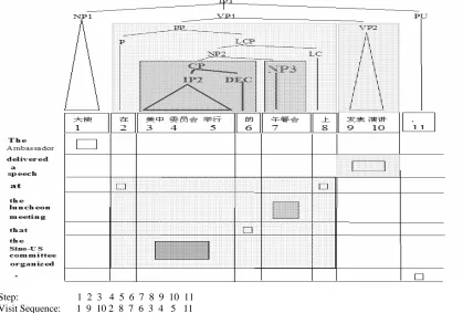
model-Step: 1 2 3 4 5 6 7 8 9 10 11 Visit Sequence: 1 9 10 2 8 7 6 3 4 5 11

Figure 1. A Chinese-English Parallel Sentence with Chinese Parse

ing the absolute source position vj, we model the jump from the last source position vj-1. All features share two common components: j (for jump), and cov (for coverage). Jumps are bucketed and capped at 4 to prevent data sparsity. Coverage is an integer indicating the visiting status of the words between the jump. Coverage is 0 if none of the words was visited prior to this step, 1 if all were visited, and 2 if some but not all were visited. (j, cov) are present in all features and are removed from the descriptions below. A couple of features use a variation of Jump and Coverage. These will be described in the feature description.

3.2 Parse-based Syntax Features

We use the sentence pair in Figure 1. as a work-ing example when describwork-ing the features. Shown in the figure are a Chinese-English parallel sen-tence pair, the word alignments between them, and

the Chinese parse tree. The parse tree is simpli-fied. Some details such as part-of-speech tags are omitted and denoted by triangles. The first step is to determine the source visit sequence from the word alignment, also shown at the bottom of

Fig-ure 1. If a target is aligned to more than one source, we assume the visit order is left to right. In Figure 1, source words 2 and 8 are aligned to the English ‘at’ and we define the visit sequence to be 8 following 2.

Chinese and English differ in the positioning of the modifiers. In English, non-adjectival modifiers follow the object they modify. This is most prominent in the use of relative clauses and prepo-sitional phrases. Chinese in contrast is a pre-modification language where modifiers whether adjectival, clausal or prepositional typically pre-cede the object they modify. In Figure 1., the Chinese prepositional phrase PP (in lightly shaded box in the parse tree) spanning range [2,8] pre-cedes the verb phrase VP2 at positions [9,10]. These two phrases are swapped in English as shown by the two lightly shaded boxes in the alignment grid. The relative clause CP (in dark

The phenomenon for the reordering model to capture is that node VP1’s two children PP and VP2 (lightly shaded) need to be swapped regard-less of how long the PP phrase is. This is also true for node NP2 whose two children CP and NP3 (dark shaded) need to be reversed.

Parse-based features model how to reorder the constituents in the parse by learning how to walk the parse nodes. For every non-unary node in the parse we learn such features as which of its child is visited first and for subsequent visits how to jump from one child to another. For the treelet VP1 PP VP2 in Figure 1, we learn to visit the child VP2 first, then PP.

We now define the notion of ‘node visit’. When a source word si is visited at step j, we find its path to root from the leaf node denoted as PathToRooti. We say all the nodes contained in PathToRooti are being visited at that step. Parse-based features are applied to every qualifying node in PathToRooti. Unary extensions do not qualify and are ignored. Since part-of-speech tags are unary branches, parse-based features apply from the lowest-level labels. Another condition depends on the jump and is discussed in section §3.4. All our features are encoded by a vector of integers and are denoted as φ (·) in this paper. We now describe the fea-tures.

3.2.1 First Child Features

The first-child feature applies when a node is vis-ited for the first time. The feature learns which of the node’s child to visit first. This feature learns such phenomena as translating the main verb first under a VP or translating the main NP first under an NP. The feature is defined as φ(currentLabel, parentLabel, nthNode, j, cov) where

currentLabel = label of the current parse node parentLabel = label of the parent node

nthNode = an integer indicating the nth occurrence of the current node

In Figure 1, when source word 9 is visited at step 2, its PathToRootis computed which is [VP2, VP1, IP1]. The first-child feature applied to VP2 is

φ(VP2, VP1, 1, 4, 1) since

currentLabel = VP2; parentLabel = VP1;

nthChild = 1: VP2 is the 1st VP among its parent’s children

j = 4: actual jump from 1 is 8 and is capped.

cov = 0: words in between the jump [1,9] are not yet visited at this step.

The semantics of this feature is that when a VP node is visited, the first VP child under it is visited first. This feature learns to visit the first VP first which is usually the head VP no matter where it is positioned or how many modifiers precede it.

3.2.2 Node Jump Features

This feature applies on all subsequent visits to the parse node. This feature models how to jump from one sibling to another sibling. This feature has these components: φ(currentLabel, parentLabel, fromLable, nodeJump,cov) where

fromLabel = the node label where the jump is from nodeJump = node distance from that node

This feature effectively captures syntactic reorder-ings by looking at the node jump instead of surface distance jump. In our example, a node-jump fea-ture for jumping from source 10 to 2 at step 4 at VP1 level is φ(PP, VP1, VP2, -1, 2) where

currentLabel = PP where source word 2 is under parentLabel = VP1

fromLabel = VP2 where source word 10 is under nodeJump = -1 since the jump is from VP2 to PP cov = 2 because in between [2,10] word 9 has been visited and other words have not.

This feature captures the necessary information for the ‘PP VP’ reorderings regardless of how long the PP or VP phrase is.

3.2.3 Jump Over Sibling Features

To make a correct jump from one sibling to the other, siblings that are jumped over should also be considered. For example in Chinese, while ing over a PP to cover a VP is a good jump, jump-ing over an ADVP to cover a VP may not be because adverbs in both Chinese and English often precede the verb they modify. The jump-over-sibling features help distinguish these cases. This feature’s components are φ(currentLabel, parent-Label, jumpOverSibling, siblingCov, j) where jum-pOverSibling is the label of the sibling that is jumped over and siblingCov is the coverage status of that sibling.

is jumped over, PP is not covered at this step, and the jump is capped to be 4.

3.2.4 Back Jump Sibling Features

For every forward jump of length greater than 1, there is a backward jump to cover those words that were skipped. In these situations we want to know how far we can move forward before we must jump backward. The back-jump-sibling feature applies when the jump is backward (distance is negative) and inspects the sibling to the right. It generates φ(currentLabel, rightSiblingCov, j). When jumping from 10 to 2 at step 4, this feature is φ(PP, 1, -4) where -4 is the jump and

currentLabel = PP where source word 2 is under rightSiblingCoverage = 1 since VP2 has been completed visited at this time. This feature learns to go back to PP when its right sibling (VP2) is completed.

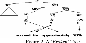
3.2.5 Broken Features

Translations do not always respect the constituent boundaries defined by the source parse tree. Con-sider the fragment in Figure 2.

Figure 2. A ‘Broken’ Tree

After the VV under VP2 is translated (“account for”), a transition is made to translate the ADVP (“approximately”) leaving VP2 partially translated. We say that the node VP2 is broken at this step. This type of feature has been shown to be useful for machine translation (Marton & Resnik 2008). Here, broken features model the context under which a node is broken by observing the feature

φ(curTag, prevTag, parentLabel, j, cov). For the transition of source word 2 to source word 1 in Figure 2, a broken feature applies at VP2: φ(AD, VV, VP2, -1 ,1). This feature learns that a VP can be broken when making a jump from a verb (VV) to an adverb (AD).

3.3 Non-Parse Features

Non-parse features do not use or use less fine-grained information from the parse tree.

3.3.1 Barrier Features

Barrier features model the intuition that certain words such as punctuation should not move freely. This phenomenon has been observed and shown to be helpful in (Xiong et. al., 2008). We call these words barrier words. Barrier features are φ (barri-erWord, cov, j). All punctuations are barrier words.

3.3.2 Number of Zero Islands Features

Although word reorderings can involve words far apart, certain jump patterns are highly unlikely. For example, the coverage pattern ‘1010101010’ where every other source word is translated would be very improbable. Let the right most covered source word be the frontier. For every jump, the number-of-zero-islands feature computes the num-ber of uncovered source islands to the left of the frontier. Additionally it takes into account the number of parse nodes in between. This feature is

defined as φ(numZeroIslands, j,

num-ParseNodesInBetween). The number of parse nodes is the number of maximum spanning nodes in between the jump. The jump at step 2 from source 1 to 9 triggers this number-zero-island fea-ture φ(1, 4, 1). The source coverage status at step 2 is 10000000100 because the first source word has been visited and the current visit is source 9. All words in between have not been visited. There is 1 contiguous sequence of 0’s between the first ‘1’ and the last ‘1’, hence the numZeroIslands = 1. There is one parse node PP that spans all the source words from 2 to 8, therefore the last argu-ment to the feature is 1. If instead, the transition was from source 1 to 8, then there would be 2 maximum spanning parse nodes for source [2,7] which are nodes P and NP2. The feature would be

φ(1, 4, 2). This feature discourages scattered jumps that leave lots of zero islands and jump over lots of parse nodes.

3.4 Training

statistics are shown in Table 1. We use the (Levy and Manning 2003) parser on Chinese.

Data #Sentences #Words

LDC2006E93 10,408 230,764

LDC2008E57 11,463 194,024

Table 1. Training Data

From the word alignments we first determine the source visit sequence. Table 2 details how the visit sequence is determined in various cases.

Alignment Type S-T Visit Sequence

1-1 Left to right from target

m-1 Left to right from source

1-m Left most target link

Ø Attaches left

Table 2. Determining visit sequence

The first column shows alignment type from source (S) to target (T). 1-1 means one source word aligns to one target word. m-1 means many source words align to one target and vice versa. Ø means unaligned source words.

After the source visit sequence is decided, fea-tures are generated. Note that the height of the tree is not uniform for all the words. To preserve the structure and also alleviate the depth problem, we use the lowest-level-common-ancestor approach. For every jump, we generate features bottom up until we reach the node that is the common ances-tor of the origin and the destination of the jump. In Figure 1 there is a jump from source 7 to 6 at step 7. The lowest-level-common-ancestor for source 6 and 7 is the node NP2 and features are generated up to the level of NP2. Features on this training data are shown in the second column in Table 5.

The MaxEnt model on this data is efficiently trained at 15 minutes per iteration (24 sen-tences/sec or 471 words/sec).

4 Experiments

4.1 Reorder Evaluation

To evaluate how accurate the reordering model is, we first compute its prediction accuracy. We choose the first 100 sentences from NIST MT03 as our test set for this evaluation. We manually word align them to the first set of reference using LDC annotation guidelines version 1.0 of April 2006.

An average of 73% of the training sentences con-tain unaligned source words and over 87% of the test sentences contain unaligned source words. The unaligned source words are mostly function words. Because the visit sequence of unaligned source words are determined not by truth but by heuristics (Table 2), they pose a problem in evalua-tion.

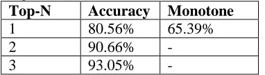
We thus evaluate the model by measuring the ac-curacy of its decision conditioned on true history. We measure performance on the model’s top-N choices for N = 1,2, and 3. Results are in Table 3. The table also shows the accuracy of no reorder-ing in the Monotone column.

Top-N Accuracy Monotone

1 80.56% 65.39%

2 90.66% -

3 93.05% -

Table 3. Reordering model performance

Figure 3 plots accuracy vs. MaxEnt training itera-tion. Accuracy starts low at 74.7% and reaches is highest at iteration 8 and fluctuates around 80.5% thereafter.

71 72 73 74 75 76 77 78 79 80 81

1 2 3 4 5 6 7 8 9 10 11 12 13 14 15

Figure 3. Accuracy vs. MaxEnt Training Iteration

We analyze 50 errors from the top-1 run. The er-rors are categorized and shown in Table 4.

Error Category Percentage

Lexical 34%

Parse 30%

Model 20%

Reference 16%

Table 4. Error Analysis

Refer-ence category are those that are marked wrong be-cause of the particular English reference. The pro-posed reorderings are correct but they don’t match the reference reorderings. Another 30% of the er-rors are due to parsing erer-rors. The Model erer-rors are due to two sources. One is the depth problem mentioned above. Local statistics for some very deep treelets overwhelm the global statistics and local jumps win over the long jumps in these cases. Another problem is the data sparseness. For ex-ample, the model has learned to reorder the ‘PP VP’ structure but there is not much data for ‘PP ADVP VP’. The model fails to jump over PP into ADVP.

4.2 Feature Utility

We conduct ablation studies to see the utilities of each feature. We take the best feature set which gives the performance in Table 3 and takes away one feature type at a time. The results are in Table 5. The first row keeps all the features. The Sub-tract column shows performance after subSub-tracting each feature while keeping all the other features. The Add column shows performance of adding the feature. Using just first-child features gets 75.97%. Adding node-jump features moves the accuracy to 78.40% and so on.

Features #Features

Sub-tract

Add

- 80.56% -

First Child 7,559 79.87% 75.97%

Node Jump 6,334 79.52% 78.40%

JumpOver Sib. 2,403 80.52% 79.00%

BackJump 602 80.48% 79.05%

Broken 15,183 80.30% 79.13%

Barrier 158 80.26% 79.22%

NumZ Islands 200 79.52% 80.56%

Table 5. Ablation study on features

5 Translation Experiments

5.1 Reorder Lattice Generation

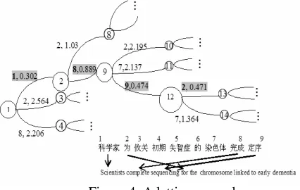
The reordering model is used to generate reorder lattices which are used by machine translation de-coders. Reorder lattices have been frequently used in decoding in works such as (Zhang et. al 2007, Kumar et.al. 2005, Hildebrand et.al. 2008), to name just a few. The main difference here is that our lattices encode probabilities from the reorder-ing model and are not used to preorder the source.

The lattice contains reorderings and their cost (negative log probability). Figure 4 shows a reor-der lattice example. Nodes are lattice states. Arcs store source word positions to be visited (trans-lated) and their cost and they are delimited by comma in the figure. Lower cost indicates better choice. Figure 4 is much simplified for readability. It shows only the best path (highlighted) and a few neighboring arcs. For example, it shows source words 1, 2, and 8 are the top 3 choices at step 1. Position 1 is the best choice with the lowest cost of 0.302 and so on.

Figure 4. A lattice example

The sentence is shown at the bottom of the figure. The first part of the reference (true) path is indi-cated by the alignment which is source sequence 1, 8, 9, and 2. We see that this matches the lattice’s top-1 choice.

Lattice generation takes source sentence and source parse as input. The lattice generation proc-ess makes use of a beam search algorithm. Every node in the lattice generates top-N next possible positions and the rest is pruned away. A coverage vector is maintained on each path to ensure each source word is visited exactly once. A wide beam width explores many source positions at any step and results in a bushy lattice. This is needed for machine translation because the parses are er-rorful. The structures that are hard for MT to reor-der are also hard for parsers to parse. Labels criti-cal to reordering such as CP are among the least accurate labels. Overall parsing accuracy is 83.63% but CP accuracy is 73.11%. We need a wide beam to include more long jumps to compen-sate the parsing errors.

5.2 Machine Translation

of using distance-based reordering and using maxi-mum entropy reordering lattices. The decoder is a log-linear phrase based decoder. Translation mod-els are trained from HMM alignments. A smoothed 5-gram English LM is built on the Eng-lish Gigaword corpus and EngEng-lish side of the Chi-nese-English parallel corpora. In the experiments, lexicalized distance-based reordering allows up to 9 words to be jumped over. MT performance is measured by BLEUr4n4 (Papineni et.al. 2001).

The test set statistics and experiment results are show in Table 6. Decoding with MaxEnt reorder lattices shows significant improvement for all con-ditions.

Data #Segs Lex

Skip-9

Reord Lattice Gain

MT03 919 0.3005 0.3315 +3.1

MT04 1788 0.3250 0.3388 +1.38

MT05 1082 0.2957 0.3236 +2.79

Table 6. MT results

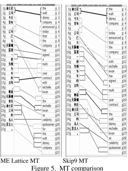
Figures 5 shows an example from MT output with word alignments to the Chinese input. The MaxEnt reordering model correctly reorders two source modifiers at source positions 8 and 22. The Skip9 output reorders locally whereas the MaxEnt lattice output shows much more complex reorder-ings.

6 Conclusions

We present a direct syntax-based reordering model that captures source structural information. The model is capable of handling reorderings of arbi-trary length. Long-range reorderings are essential in translation between languages with great word order differences such as Chinese-English and Arabic-English. We have shown that phrase based SMT can benefit significantly from such a reorder-ing model.

The current model is not regularized and feature selection by thresholding the feature counts is quite primitive. Regularizing the model will prevent overfitting, especially given the small training data set. Regularization will also make the ablation study more meaningful.

The reordering model presented here aims at capturing structural differences between source and target languages. It does not have enough lexical features to deal with lexical idiosyncrasies.

ME Lattice MT Skip9 MT

Figure 5. MT comparison

Our initial attempt at adding lexical pair jump fea-tures φ(fromWord, toWord, j) has not proved use-ful. It hurt accuracy by 3% (from 80% to 77%). We see from Table 4 that 34% of the errors are due to source lexical choices which indicates the weak-ness of the current lexical features. Regularization of the model might also make a difference with the lexical features.

Reordering and word choice in translation are not independent of each other. We have shown some initial success with a separate reordering model. In the future, we will build joint models on reordering and translation. This approach will also address some of the reordering problems due to source lexical idiosyncrasies.

7 Acknowledgement

We would like to acknowledge the support of DARPA under Grant HR0011-08-C-0110 for fund-ing part of this work. The views, opinions, and/or findings contained in this article are those of the author and should not be interpreted as represent-ing the official views or policies, either expressed or implied, of the Defense Advanced Research Projects Agency or the Department of Defense.

A.S.Hildebrand, K.Rottmann, Mohamed Noamany, Qin Gao, S. Hewavitharana, N. Bach and Stephan Voga. 2008. Recent Improvements in the CMU Large Scale

Chinese-English SMT System. In Proceedings of

ACL 2008 (Short Papers)

C. Wang, M. Collins, and Philipp Koehn. 2007.

Chi-nese Syntactic Reordering for Statistical Machine Translation. In Proceedings of EMNLP 2007

Chi-Ho Li, Dongdong Zhang, Mu Li, Ming Zhou, Minghui Li, and Yi Guan. 2007. A Probabilistic

Approach to syntax-based Reordering for Statistical Machine Translation. In Proceedings of ACL 2007.

Christoph Tillmannn. 2004. A Block Orientation

Model for Statistical Machine Translation. In

Pro-ceedings of HLT-NAACL 2004.

David Chiang. 2005. A Hierarchical Phrase-based

Model for Statistical Machine Translation. In

Pro-ceedings of ACL 2005.

Dekai Wu. 1997. Stochastic Inversion Transduction

Grammars and Bilingual Parsing of Parallel Cor-pora. Compuntational Linguistics, Vol. 23, pp

377-404

Deyi Xiong, Qun Liu, and Shouxun Lin. 2006.

Maxi-mum Entropy Based Phrase Reordering Model for Statistical Machine Translation. In Proceedings of

ACL 2006.

Deyi Xiong, Min Zhang, Aiti Aw, Haitao Mi, Qun Liu and Shouxun Lin. 2008. Refinements in FTG-based

Statistical Machine Translation. In Proceedings of

ICJNLP 2008

Dongdong Zhang, Mu Li, Chi-Ho Li, and Ming Zhou. 2007. Phrase Reordering Model Integrating

Syntac-tic Knowledge for SMT. In Proceedings of EMNLP

2007

Fei Xia and Michael McCord. 2004. Improving a

Sta-tistical MT System with Automatically Learned Re-write Patterns. In Proceedings of COLING 2004.

Franz Josef Och and Hermann Ney. 2004. The

Align-ment Template Approach to Statistical Machine Translation. Computational Linguistics, Vol. 30(4).

pp. 417-449

Kenji Yamada and Kevin Knight 2001. A Syntax-based

Statistical Translation Model. In Proceedings of

ACL 2001

Kevin Knight. 1999. Decoding Complexity in Word

Replacement Translation Models. Computational

Linguistics, 25(4):607-615

Kishore Papineni, Salim Roukos, Todd Ward, and Wei-jing Zhu. 2001. A Method for Automatic Evaluation

for MT. In Proceedings of ACL 2001

Michael Collins, Philipp Koehn, and Ivona Kucerova. 2005. Clause Restructuring for Statistical Machine

Translation. In Proceedings of ACL 2005.

Michell Galley, Christoph D. Manning. 2008. A Simple

and Effective Hierarchical Phrase Reordering Model. Proceedings of the EMNLP 2008

Perter F. Brown, Stephen A. Della Pietra, Vincent J. Della Pietra, and Robert L. Mercer. 1993. The

Mathematics of Statistical Machine Translation.

Computation Linguistics, 19(2).

Philip Koehn, Franz Josef Och, and Daniel Marcu. 2003. Statistical Phrase-based Translation. In Pro-ceedings of NLT/NAACL 2003.

Richard Zens, Hermann Ney, Taro Watanabe, and Eii-chiro Sumita. 2004. Reordering Constraints for

Phrase-based Statistical Machine Translation. In

Proceedings of COLING 2004.

Richard Zens and Hermann Ney. 2006. Discriminative

Reordering Models for Statistical Machine Transla-tion. In Proceedings of the Workshop on Statistical

Machine Translation, 2006.

Roger Levy and Christoph Manning. 2003. Is it harder

to parse Chinese, or the Chinese Treebank? In

Pro-ceedings of ACL 2003

Shankar Kumar and William Byrne. 2005. Local

Phrase Roerdering Models for Statistical Machine Translation. In Proceedings of HLT/EMNLP 2005

Stephan Kanthak, David Vilar, Evgeny Matusov, Rich-ard Zens, and Hermann Ney. 2005. Novel

Reorder-ing Approaches in Phrase-based Statistical Machine Translation. In Proceedings of the Workshop on

Building and Using Parallel Texts 2005.

Y. Al-Onaizan . K. 2006 Distortion Models for

Statisti-cal Machine Translation. In Proceedings of ACL

2006.

Yizhao Ni, C.J.Saunders, S. Szedmak and M.Niranjan 2009 Handling phrase reorderings for machine

translation. In Proceedings of ACL2009

Yuqi Zhang, Richard Zens, and Hermann Ney. 2007.

Improved Chunk-level Reordering for Statistical Ma-chine Translation. In Proceedings of HLT/NAACL

2007.

Yuval Marton and Philip Resnik. 2008. Soft Syntactic