Conflict detection and analysis for single-pushout high-level replacement

(1)

Formal Methods and Tools

Faculty of Electrical Engineering, Mathematics and Computer Science

Master Thesis

Conflict Detection and Analysis

for Single-Pushout High-Level

Replacement

Author:

Ruud Welling

Committee:

prof.dr.ir. Arend Rensink

dr. Peter van Rossum

dr.ir. Jan Kuper

(2)

Abstract

In many graph transformation systems (local) confluence is a desired property. For instance, if graph transformation is used for model transformation, then confluence and termination ensure that the order in which rules are applied does not matter, in other words, the final result will always be the same. In this research we investigate sufficient conditions for local confluence of high-level replacement (HLR) systems. Using the single-pushout high-level replacement approach we define critical pairs (minimal conflicting situations). Our sufficient condition for local confluence is based on the analysis of critical pairs. We provide our proofs on a categorical level, therefore our theory cannot only be applied to the category of graphs: we formulate requirements for the categories for which our theorems hold, and we show that our theory is also applicable to attributed graphs.

We also present some of the foundations for confluence analysis for HLR systems with negative application conditions (NACs). In order to show local confluence for a HLR system with NACs we will show that stricter conditions must hold for the critical pairs with NACs (compared to the situation with-out NACs). We show that HLR systems withwith-out NACs are locally confluent. Further analysis of HLR systems with NACs is future work.

(3)

Chapter 1

Introduction

In today’s world, models exist to help us represent and understand many things. For example, maps or blueprints can model the world or a building. In com-puter science, graphs are used as models almost everywhere; for example, data and control flow diagrams, UML diagrams, Petri nets, and hardware and soft-ware architectures are usually visualized with graphs. Many softsoft-ware develop-ment approaches use graphs to model software under developdevelop-ment [21, 28]. In this area of model-based software development processes, we are witnessing a paradigm shift, models are no longer mere (passive) documentation, but they are used for code generation, analysis, and simulation as well [18]. Because so many models in software engineering can be represented as graphs, we can use graph transformation as a formalism to specify model transformation.

Graph grammars and graph transformations originated in the early 1970’s [4, 7, 15, 29, 30, 34]. Since then the list of areas where graph grammars and transformations have been useful has grown impressively: pattern recognition [37], compiler construction [1], software specification and development [16], database design [20], modelling of concurrent systems [17], visual languages [3] and many others [36]. This wide applicability is due to the fact that graphs are a very natural way of explaining complex situations on an intuitive level. Graph transformation allows us to model the dynamics in these descriptions, since it can describe the evolution of graphical structures [10]. Graph trans-formation can also be useful if no (system) dynamics are involved, for example in case graph transformations transform one model into another. For model transformations, we can use the theory of graph transformation to verify the correctness of these transformations [11, 12].

1.1

What is Graph Transformation

(6)

The changes in graph transformations are guided by rules (also called pro-duction rules). Rules specify changes in a relatively small substructure of a graph; these changes are modifications to that substructure, such as adding or removing certain parts from the substructure.

The most important requirement for a rule to apply is the occurrence of the substructure in the host graph. We call this substructure theleft-hand side (LHS) of the rule. An occurrence of the LHS in a host graph is called amatch. A rule also has aright-hand side (RHS) which (partially) overlaps with the LHS. All vertices and edges that are both in the LHS and RHS are preserved after applying the rule. The LHS can have vertices and edges which are not in the RHS, these are the vertices and edges that are deleted by the rule. The RHS can also have vertices and edges that are not in the LHS, these vertices and edges are created after applying rule.

It is possible for a rule to havenegative application conditions (NACs), which can restrict applicability of a rule. A NAC is a graph that partially overlaps with the LHS of the rule. When a match for a rule exists, the rule is a candidate for application, however the rule may not be applied if one of the NACs of the rule is not satisfied. A NAC is satisfied when there does not exist an occurrence of the NAC in the host graph such that the overlapping part of the NAC and the LHS also overlap in the occurrence of the LHS (the match) and the occurrence of the NAC in the host graph

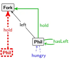
Figure 1.1 shows a rule with a NAC. This rule models a philosopher (Phil) which grabs a Fork on his left. The rule is applicable to some host graph G

if Gcontains a Phil-vertex with has ahungry-self-edge and a left-edge to a

Forkvertex, however there may not exist aPhil-vertex which has ahold edge to the same Fork. If there does exist such a vertex, the NAC is not satisfied.

In Figure 1.2 we show the same rule without the NAC, the graph Lis the left-hand side of the rule, andRis the right-hand side. The rule can be applied to the graph G, the occurrence ofL inGis shown by the dotted lines. We can see that the NAC is satisfied because there exists no holds-edge which targets the bottom fork inG.

The application of the rule results in the graphH. We can see that the rule deletes thehungry-edge of the right philosopher. The rule also adds two edges, namely an hasLeft-self-edge, and ahold edge. We can see that the topFork

and the leftPhilwere not needed by the rule. These vertices are left untouched in the resulting graphH.

A graph transformation system (GTS) consists of a set of rules. When a rule is applicable to a graphG, and application of this rule gives the graphH, then we say that G can be directly transformed to H. A transformation can consist of multiple steps: ifGcan be (directly) transformed toH andH can be (directly) transformed toX, then we say thatGcan betransformed toX.

1.2

Approaches to Graph Transformation

(7)

Phil

Phil Fork

hungry hold

left

hold

hasLeft

Figure 1.1: A Rule with a NAC. The LHS, RHS and the NAC are shown as one graph: the thin and dashed (blue) edge (hungry) is in the LHS and NAC, but not in the RHS; the wide (green) edges are in the RHS but not in the LHS or NAC; the thick dashed (red) edges and vertices are in the NAC, but not in the LHS or RHS. All other vertices and edges are in the NAC, LHS and RHS. The textsPhil andFork on the vertices can be considered self-edges with the text as a label.

Phil

Fork Fork

Phil Phil

Fork Fork

Phil

Fork

Phil

Fork

Phil

hasLeft

hungry left

hungry

left left

hasLeft

left

right

right hungry

hungry left

right

hold hold

L R

G H

(8)

Two common algebraic approaches to graph transformation are the double-pushout (DPO) approach and the single-double-pushout (SPO) approach. There are two cases where these approaches yield different results.

• When a rule has a match, but straightforward application of the rule would leave a dangling edge (an edge from which either the source or target vertex has been deleted), the result is no longer a proper graph (since every edge needs a source and a target vertex). Both approaches solve this differently.

• When a rule is applied via a non-injective match (i.e., two verticesv1 and

v2 of the LHS are matched onto one vertex v of the host graph), and the rule deletes one of these vertices, but keeps the other, a complicated situation arises where the two approaches choose a different solution.

For both cases the rule would not be applicable in the DPO approach, whereas the SPO approach prioritizes the deletion: in the first case the dangling edge is deleted, and in the second case the vertex v of the host graph will be deleted (with all incident edges). A detailed presentation and comparison of the SPO and DPO approaches can be found in [13].

High-Level Replacement

The SPO approach (as well as other algebraic approaches) relies heavily on cat-egory theory. This approach cannot only be used to transform graphs, but also other structures. The transformation of these structures is also calledhigh-level replacement. A transformation system using high-level replacement is called a high-level replacement system (HLR system). A graph transformation system is an example of an HLR system.

We will prove our theorems on a categorical level; in order to do so we define SPO categories, SPO categories fulfil several requirements which allow us to prove our theorems. We will show that there exists an SPO category for transformation of graphs, and we will show that our results can also be applied to attributed graphs. It is very likely that our work can be extended to allow transformation of other structures such as typed graphs, hypergraphs or Petri nets.

1.3

Conflicts and Confluence

Graph transformation is commonly used for model transformation. When trans-forming models it is important that there exists exactly one final result. Given an HLR system, where the objectG(such an object could be a graph) can be transformed to some objectX, we say thatX is anormal form ofGif no rules in the HLR system can be applied to X. If every object has a unique normal form, then the order in which rules are applied does not matter.

(9)

then there must exist an object Z and transformations formX to Z and from

Y toZ. Confluence ensures that there exists at most one normal form [8]. A weaker version of confluence is calledlocal confluence. An HLR system is locally confluent if for all pairs of direct (single-step) transformations from an objectGtoH1 and fromGtoH2, there is an objectX such that bothH1 and

H2can be transformed toX after applying any number of rules.

We say that an HLR system is terminating when there do not exist infinite transformation sequences. If an HLR system is locally confluent and terminat-ing, then the HLR system is confluent [8]. The termination also ensures the existence of a normal form. Therefore a locally confluent and terminating HLR system has a unique normal form for every object.

It is a known fact that (local) confluence is an undecidable problem [31, 33]. It is also known that termination of an HLR system is undecidable [32]. Some termination criteria for graph transformation systems have been shown in [9].

In this research we will investigate sufficient conditions for when an HLR sys-tem is locally confluent. In order to investigate whether an HLR syssys-tem is locally confluent, we need to study conflicts: given a pair of rules with matches into the same host object, the transformations induced by two rules with matches are in conflict when after application of one of the rules, the other can no longer be applied with the same match.

Conflict detection is an important part of our research. We want to find out which pairs of rule applications can be used independently and which cannot. We can distinguish two different kinds of conflicts.

• The most basic kind of conflict is the delete-use conflict. This type of conflict can occur in any HLR system. A pair of rules is in delete-use conflict when one rule deletes something that was in the match of the other rule. In other words, a part of the host object that was needed by the second rule was deleted by the first rule, and therefore the second rule can no longer be applied via the same match.

• When we have rules with NACs in our HLR system, a conflict may arise where one rule adds some structure to the host object that is forbidden by the NAC of the other rule. We call this conflict aproduce-forbid conflict.

The problem of conflict detection has been studied in some depth for the DPO approach [19, 24, 25, 26]. In this thesis we want to extend the existing results for DPO high-level replacement to the SPO setting.

In order to analyse conflicts efficiently, we search for conflict situations where the host object is as small as possible. We call this acritical pair.

Critical pairs are useful because (as we prove) there exists a critical pair for every conflict. Therefore critical pairs can be used to reason about all conflicts in an HLR system. We will show that an HLR system is locally confluent when all critical pairs fulfil a slightly stricter definition of local confluence.

1.4

Graph Transformation Tools

(10)

in _groove. _Agg is an interesting tool because it already supports conflict detection, however it can only detect conflicts for DPO graph transformation.

The two tools are similar in the sense that they can both model graph transformation systems. Both tools allow users to create graph transformation rules and apply these to a host graph.

Agg(the Attributed Graph Grammar system) is a general development en-vironment for algebraic graph transformation systems. _Agg supports several kinds of validations. Theagggraph parser is able to check if a graph belongs to a certain graph language determined by a graph grammar. Aggcan check con-sistency conditions that describe basic properties of graphs such as the existence of certain elements. aggcan also perform critical pair analysis, for each pair of rules agg can find a minimal examples representing all conflicting situations. [38]

Groove(GRaph based Object-Oriented VErification) is a graph transfor-mation tool for software model checking of object-oriented systems. _Groove is able to generate the state space given a start graph and a set of rules. This allows _groove perform LTL and CTL model checking: _groove can check whether certain properties hold for all states. [35]

1.5

Related Work

A lot of research on conflict detection using DPO graph transformation has already been done: an efficient method to compute the set of all critical pairs for a graph transformation system has been proposed in [25]. This work is continued in [26] where the author defines essential critical pairs as a subset of critical pairs. Critical pair detection for graph transformation rules with NACs has been discussed in [23, 24]. A method for conflict detection for typed attributed graph transformation system is proposed in [19].

Many important concepts for the SPO transformation have been described by Ehrig et al. [13]; for instance, the concept of parallel independence, but also an embedding theorem, which we need later to show that local confluence of all critical pairs implies local confluence of the graph transformation system. SPO graph transformation for attributed graphs is also discussed.

Some work on SPO high-level replacement systems has been done by Ehrig et al. [14]. Ehrig defines some requirements for categories which can be used for SPO high-level replacement. Furthermore, parallel independence is defined, and local confluence of parallel independent transformations is shown.

For SPO graph transformation, L¨owe [27] proves that a GTS is locally fluent if every critical pair is strictly confluent (also called transformation con-fluent). Strict confluence is stronger than local confluence, the author explains why local confluence of all critical pairs is not sufficient to show that a GTS is locally confluent. This paper does not show completeness of critical pairs, and the proof for the local confluence theorem is not completely clear.

1.6

Research Questions

(11)

extend these methods so they can be used in the single-pushout approach. Our final goal is to implement an algorithm for critical pair detection and conflu-ence analysis in_groove. To reach this goal, we have broken it down into the following sub-questions:

1. How can the existing theory on finding critical pairs using the double-pushout approach be modified for the single-double-pushout approach?

2. How can we implement an algorithm to find critical pairs?

3. For which cases can we determine if a critical pair is locally confluent?

1.6.1

Modifying existing theory

The first important step is to come up with a definition for critical pairs and prove that the local confluence of all critical pairs implies the local confluence of an HLR system.

Our proofs are on an abstract categorical level: we define SPO categories, and prove our results for these SPO categories. Therefore our results are not only applicable for transformation of graphs. We will show that we can also apply our results to attributed graphs. And it is very likely that our results can also be applied to other structures.

Validation After every step, we will provide formal proofs to show that our results are correct. We will show completeness of critical pairs and we will show that the (strict) confluence of all critical pairs implies local confluence of the graph transformation system.

1.6.2

Algorithm for Critical Pair Detection

Our second research question goes well together with our first question. Based on the definition we have given for critical pairs, it was easy to come up with a method to compute all critical pairs for a graph transformation system. We have implemented this in an algorithm for_groove.

Validation In order to test whether our algorithm is correct, we have reused some existing test cases for critical pair detection which have been implemented in _agg. Since it is unclear whether the critical pair test cases for_aggare only for DPO critical pairs, we will have to build some SPO-specific test cases.

1.6.3

Determining local confluence

(12)

Validation We cannot decide local confluence for all cases. However we can test our implementation on some of the many graph transformation systems that are (supposedly) confluent that have already been implemented in_groove. We can then see how well we can decide confluence in practice.

1.7

A Last Minute Result

Just before finishing this thesis, we have discovered that pushouts (transforma-tions) do not always exist in the category of simple graphs. The counterexample (which we present in Appendix A.2) shows that a situation in which our pushout construction (which defines how a graph is transformed) is not correct in all sit-uations.

Because of this some of our propositions about graphs are no longer valid. Our main proofs, however, are proven using abstract categories, for which we have defined the properties required for the results to hold; the fact that the category of simple graphs turns out not to satisfy those properties in no way invalidates the results. For those propositions and proofs which are not valid, we have added footnotes which state that this is the case. A more careful analysis of the situation can be found in Section 8.3.

1.8

Structure

Chapter 2 will explain the basics of our work. We will formally define graphs, provide an introduction to category theory, and we will show how objects (such as graphs) can be transformed to other objects using high-level replacement.

In Chapter 3 we will define the concept of critical pairs and prove that the (strict) local confluence of all critical pairs implies the local confluence of the high-level replacement system. Most of the concepts we introduce in this section already existed (for example for the DPO approach or for SPO graph transformation), however the proofs in this section are all new work.

Chapter 4 will introduce rules with NACs. We will extend the definition for critical pairs to allow rules with NACs, and we will show a sufficient condition for when a high-level replacement system is locally confluent, however we believe a better sufficient condition may be found in the future. The concept of NACs has already been defined by Ehrig et al. [13], however to our knowledge no research has been done on critical pair analysis for SPO high-level replacement (or graph transformation) with NACs.

In Chapter 5 we will define attributed graphs. This definition is based on the existing definition given by Ehrig et al. [10]. We will also show that the theory we have developed in the previous chapters is applicable to attributed graphs.

In Chapter 6 we will show that the local confluence of one critical pair can imply the local confluence of a second critical pair. This can be used as an alternative method to decide local confluence of a critical pair.

(13)

Chapter 2

High-Level Replacement

and Graph Transformation

Systems

This chapter will introduce what graph transformation is and how it works. We start by defining what graphs and graph morphisms are in Section 2.1. Graph transformation relies heavily on category theory. In fact, the single-pushout approach does not only allow transformation of graphs, but also other kinds of objects, such as sets and attributed graphs. Because of this we will explain how to transform objects in any category (for which certain requirements must hold). We will cover the basics of category theory in Section 2.2. In Section 2.3 we will explain how we can apply a rule to an object, to transform it into another object. In Section 2.4 we will define transformation systems for any kind of object (called high-level replacement systems), we will also state the requirements for categories which can be used in SPO high-level replacement systems.

2.1

Graphs and Morphisms

The theory that we develop in this research will be applied in the context of graphs. Even though our proofs are generalized so they can also be applied to different objects, we will be using graphs as examples to make it clear how our theory can be applied to graphs. We start by formally defining what a graph is. We will be using graphs with labelled edges; these labels are elements ofLab which is the universe of all possible labels.

Definition 2.1.1 (Graph and Subgraph). A graph is a tuple G = (VG, EG)

consisting of a setVG of vertices, and a set EG⊆VG×Lab×VG of (directed)

edges. Given an edge e = (v1, a, v2) ∈ EG, the source and target mappings

sG, tG:EG→VG and label mappinglG:EG→Lab are defined bysG(e) =v1,

(14)

Remark. Using this definition of graphs, we ensure that every pair of vertices can be connected by at most one (directed) edge with a given label.

Now given two graphs, we want a way to specify how one graph relates to the other. For this we use mappings between the sets of vertices and edges. We will first define mappings for sets.

Definition 2.1.2 (Mappings between Sets). Apartial mapping f from a setA

to a setB, denotedf :A→B, maps elements ofAto elements of B.

• We say thatf isinjective if for all a, a0∈A,f(a) =f(a0) impliesa=a0,

• We say thatf issurjectiveif for allb∈Bthere is anasuch thatf(a) =b

• We say thatf istotal iff is defined for alla∈A

• Every mappingf :A→B is a total mapping from some subset dom(f) ofAtoB. We call dom(f) thedomain off.

• We will sometimes writef(A) =C, whereC={f(a)|a∈dom(f)}.

• A pair of mappings (e1, e2) withei:Ai→B for (i= 1,2) is calledjointly

surjective whene1(A1)∪e2(A2) =B.

• Two mappingsf :A→B andg:B→C can becomposed which results in a mappingg◦f :A→C, composition is defined as follows:

(g◦f)(x) =

(

g(f(x)) ifx∈dom(f) andf(x)∈dom(g)

undefined otherwise

Remark. From this definition we can conclude that composition of mappings is associative i.e., h◦(g◦f) = (h◦g)◦f, for any f : A → B, g : B → C and

h:C→D.

A mapping between two graphs, called a graph morphism, allows us to show that a graph contains a substructure of another graph.

Definition 2.1.3 (Graph Morphism). A partial graph morphism (also called graph morphism) f : G → H between two graphs G, H is a pair f = (fV :

VG →VH, fE :EG →EH) of partial mappings, such that the sources, targets

and labels are preserved for every edge, i.e.,fV◦sG =sH◦fE,fV◦tG=tH◦fE

andlG=lH◦fE.

We say that a partial graph morphismf is total (resp. injective, surjective) if bothfV andfE are total (resp. injective, surjective). Two graph morphisms

f :L →Gand g: H →G arejointly surjective if both (fV, gV) and (fE, gE)

are jointly surjective. For a partial graph morphism g we say that dom(g) = (dom(gV),dom(gE)) is the domain of g. Graph morphisms can be composed:

given f : X →Y, g : Y → Z andh: X →Z we have g◦f = (gV ◦fV, gE◦

fE) (using the associativity of function composition and the fact thatg and f

preserve sources, targets and labels, we know thatg◦f is a graph morphism as well).

(15)

The next proposition directly follows from the fact that graph morphisms preserve sources and targets.

Proposition 2.1.4. Let g : G → H be a partial graph morphism. Then dom(g) = (dom(gV),dom(gE))is a subgraph ofG.

Proof. We know that dom(g) is a graph if dom(gE)⊆dom(gV)×Lab×dom(gV),

this is the case because gV ◦ sG = sH ◦gE, gV ◦tG = tH ◦gE. We know

by definition that dom(gV) ⊆ GV and dom(gE) ⊆ GE, therefore dom(g) is a

subgraph ofG.

Many concepts for algebraic graph transformation rely on category theory. The next section will cover many basics of category theory using sets with mappings and graphs with graph morphisms as examples.

2.2

Category Theory Basics

Before diving into the detail of SPO High-Level Replacement, we introduce some basic definitions which are needed for our proofs. We will define categorical generalizations of injective, surjective and jointly surjective morphisms. These generalisations allow us to prove many of our theorems using category theory.

A large part of the definitions in this section is based on the definitions in [2, 10]. We start by defining categories.

Definition 2.2.1(Category). AcategoryC = (ObC,MorC,◦,id) is defined by • a classObC ofobjects

• for each pair of objectsA, B∈ObC, a setMorC(A, B) ofmorphisms

• for all objectsA, B, C ∈ObC, acomposition operation◦(A,B,C): MorC(B, C)×MorC(A, B)→MorC(A, C)

• for each objectA∈ObC, anidentity morphismidA∈MorC(A, A)

such that the following conditions hold:

1. Associativity. For all objects A, B, C, D∈ObC and morphisms f : A→

B, g:B →C, h:C→D it holds that (h◦g)◦f =h◦(g◦f),

2. Identity. For all objects A, B∈ObC and morphismsf :A→B, it holds thatf◦idA=f andidB◦f =f.

Remark. Instead of f ∈MorC(A, B), we writef :A →B. We also leave out the index for the composition operation, since it is clear which one to use.

In the next two definition we define two categories, one is based on sets and the other is based on graphs. In both categories the morphisms are partial mappings.

(16)

Definition 2.2.3 (CategoryGraphP₎_. _{The category} _GraphP _{consists of the} class of all graphs (as defined in Definition 2.1.1) as objects with all possible graph morphisms (see Definition 2.1.3). Composition has been defined in Defi-nition 2.1.3, and identities are the pairwise identities on the sets of vertices and edges.

Next we define monomorphisms and epimorphisms. A monomorphism is a categorical generalization of a total injective morphism, similarly an epimor-phism is a categorical generalization of a surjective morepimor-phism.

Definition 2.2.4 (Monomorphism and Epimorphism). Given a categoryC, a morphism m : B → C is called a monomorphism if, for all morphisms f, g :

A→B it holds thatm◦f =m◦g impliesf =g.

A morphism e : X → A is called an epimorphism if, for all morphisms

f, g:A→B, it holds thatf◦e=g◦eimpliesf =g.

A fg ////B m //C X e //A fg ////B

Remark. We will often say that a morphismf is mono (resp. epi) to denote that

f is a monomorphism (resp. epimorphism).

In the following lemma and propositions, we will show forSetP_{, that the} monomorphisms are the injective and total mappings, and that the epimor-phisms are the surjective mappings. Later, in Proposition 2.2.13 we show that this is also true forGraphP.

Lemma 2.2.5. Every monomorphism inSetP _{is total.}

Proof. Letm: A→B be a mapping which is not total. Then there exists an

x∈Asuch that m(x) is undefined. LetidA:A→Abe the identity morphism

ofA, and constructf :A→Aas follows:

f(a) =

(

a ifa6=x

undefined otherwise

It is clear thatf 6=idA, we also know that m◦idA=m, and by choice off we

know thatm◦f =m(since m(x) andf(x) are both undefined). Therefore we havem◦f =m◦idAbutf 6=idA, this means thatmis not a monomorphism.

Now we can prove that aSetP_{-monomorphism is equivalent to an injective} and total set mapping.

Proposition 2.2.6. A SetP_-morphism _f _:_A_→_B _{is a monomorphism if and} only if it is total and injective.

Our proof is based on a similar proof in [2].

Proof. (⇒) Letf :A→B be a monomorphism, let a, a0 ∈Asuch thata6=a0, and let{x}be a one-element set. Consider the mappingsg, g0 _:_{_x_{} →}_A_where

g(x) = a and g0(x) = a0. Sinceg 6=g0 it follows, since f is a monomorphism, that f◦g6=f◦g0, thereforef(a) = (f ◦g)(x)6= (f◦g0)(x) =f(a0). Therefore

f is injective. Lemma 2.2.5 states thatf must also be total.

(⇐) Conversely suppose thatf is total and injective, andg, h:C→A are mappings such that g6=hand for somec∈C we haveg(c)6=h(c). Sincef is injective, it follows thatf(g(c))6=f(h(c)), thereforef◦g6=f◦h, which means

(17)

Similarly we show forSetP _{that epimorphisms coincide with surjective set} mappings.

Proposition 2.2.7. A SetP_-morphism _f _: _A_→ _B _{is an epimorphism if and} only if it is surjective.

We repeat the proof given in [2].

Proof. (⇒) Suppose f :A →B is not surjective. Then there is ab ∈B such that ∀a∈A:f(a)6=b. Defineg1, g2:B → {0,1}as follows: g1(x) = 0 for all

x∈ B, and g2(x) = 1 if x=b and 0 otherwise. We have g1◦f =g2◦f but

g16=g2 thereforef is not an epimorphism.

(⇐) Conversely, supposef :A→B is surjective, and let g1, g2:B→Cbe mappings such thatg16=g2. Then there is absuch thatg1(b)6=g2(b). Because

f is surjective, b has a preimage in a ∈ A such that f(a) = b. Therefore

g1(f(a))6=g2(f(a)) andg1◦f 6=g2◦f. It follows thatf is an epimorphism.

Definition 2.2.8 (Isomorphism). A morphismi:A→B is called an isomor-phism if there exists a morphism i−1 _: _B _→ _A _{such that} _i_◦_i−1 ₌ _id

B and

i−1_◦_i₌_id

A

A i //_B i−1

o

Two objectsA andB are isomorphic, writtenA∼=B, if there is an isomor-phismi:A→B.

Remark. All the theory that is explained in this paper is supposed to work modulo isomorphism; i.e., we want to consider isomorphic objects equal.

In the category GraphP it is well known that isomorphisms are injective, total and surjective graph morphisms. We show that injective, total and sur-jective graph morphisms are indeed isomorphisms in Proposition 2.2.13. First we will show that for any category, an isomorphism is both a mono and an epi.

Proposition 2.2.9. Every isomorphism is both a monomorphism and an epi-morphism.

Proof. See [2].

The converse does not hold for every category [2], however we will show for SetP _{that an isomorphism is equivalent to a morphism which is both mono and} epi. We already know (Propositions 2.2.6 and 2.2.7) that everySetP_-morphism which is both mono and epi must be injective, total and surjective.

Proposition 2.2.10. A surjective, injective and totalSetP-morphismf :A→

B is an isomorphism.

Proof. Because f is surjective we know that for every b ∈ B there exists an

a∈Asuch thatf(a) =b, becausef is injective we know thatais unique, and because f is total we know that every element of f has an image in B. We define the morphism f−1 _:_B _→_A _{as follows for all}_b _∈_B_: _f−1₍_b_{) =}_a _where

a ∈ A such that f(a) =b. Now we have f−1₍_f₍_a_{)) =} _a _{for any} _a _∈ _A_{, and}

f(f−1₍_b_{)) =}_b_{for any}_b_∈_B_{. Therefore}_f_◦_f−1₌_id

B andf−1◦f =idA, which

(18)

The next definition defines when a pair of morphisms with the same target is called jointly epimorphic. This definition is taken from [10].

Definition 2.2.11 (Jointly Epimorphic). A morphism pair (e1, e2) with ei :

Ai →B for (i= 1,2) is calledjointly epimorphic if, for allg, h:B →C with

g◦ei =h◦ei fori= 1,2 we haveg=h:

A1 e1 ,,

B _hg ////C A2

e2 22

Next we show that this constitutes a categorical generalization of a pair of jointly surjective morphisms. Remember that we call a pair ofSetP _morphisms (e1, e2) withei :Ai→B for (i= 1,2) jointly surjective whene1(A1)∪e2(A2) =

B.

Proposition 2.2.12. A pair ofSetP_-morphisms₍_e

1, e2)with ei:Ai→B for

(i= 1,2) is jointly epimorphic if and only if it is jointly surjective.

Our proof is fairly similar to the proof of Proposition 2.2.7 which originates from [2].

Proof. (⇒) Suppose (e1, e2) are not jointly surjective. Then there is a b ∈ B such that∀a∈A1:e1(a)6=b, and∀a∈A2:e2(a)6=b. Defineg, h:B→ {0,1} as follows: g(x) = 0 for all x ∈ B, and h(x) = 1 if x = b and 0 otherwise. We have g◦ei =h◦ei for i = 1,2 but g 6= htherefore (e1, e2) is not jointly epimorphic.

(⇐) Conversely, suppose (e1, e2) is jointly surjective, and letg, h: B →C be mappings such thatg6=h. Then there is absuch thatg(b)6=h(b). Because

e1 and e2 are jointly surjective, b must have a preimage in e1 or e2. Assume (the other case is analogous)bhas a preimage ine1i.e., we have ana∈A1such thate1(a) =b. Then we knowg(e1(a))6=h(e1(a)) andg◦e16=h◦e1, therefore

e1 ande1 are jointly epimorphic.

Proposition 2.2.13. For any morphism f : A → B in either, SetP_{, or}

GraphP we have:

1. f is a monomorphism if and only if it is total and injective.

2. f is an epimorphism if and only if it is surjective.

3. f is an isomorphism if and only if it is total, injective and surjective.

4. Let g : A0 → B be a morphism in the same category as f, then the pair (f, g)is jointly epimorphic if and only if it is jointly surjective.

Proof. We have already shown these properties forSetP_{-morphisms in} Propo-sitions 2.2.6, 2.2.7, 2.2.9, 2.2.10 and 2.2.12.

Recall (Definition 2.1.3) that aGraphP_-morphism_f _{is total (resp. injective,} surjective) iffV andfEare total (resp. injective, surjective). A pair ofGraphP

-morphismsf, f0 with the same target is jointly surjective if both pairs (fV, fV0 )

and (fE, fE0 ) are jointly surjective. Now we can conclude that all properties of

(19)

2.3

Transformation by Pushout

In high-level replacement systems (HLR systems) objects are transformed to other objects. The changes in these transformations are guided by rules. Every rule has a morphism (the rule morphism) which belongs to a special subclass R of rule morphisms. In the category GraphP we can use any partial graph morphism as a rule morphism, i.e., R contains all GraphP-morphisms. For some categories however, not all morphisms are allowed to be rule morphisms: in Chapter 5 we will see that we cannot use every AGraphP-morphism to transformAGraphP objects.

The definition presented here is applicable to any category C. Later on, when we define SPO HLR systems in Section 2.4, we will specify what conditions must hold the categoryC and the class of morphismsR.

Definition 2.3.1 (Rule). Given a category C with a class R of morphisms, a rule (also called production) p = (L −→r R) is an R-morphism, called the rule morphism. The objects L and R are called theleft-hand side (LHS) and right-hand side (RHS) ofp, respectively.

Remark. The rules we have defined here are simple rules. For now we consider only these simple rules. Later, in Chapter 4 we will cover rules with negative application conditions (NACs).

In order to be able to apply a rulep= (L−→r R) to a objectG, we need an occurrence of the left-hand side of the rule inG. This occurrence is defined by a morphismm:L→Gsuch thatmbelongs to a class of match-morphismsM. The exact requirements on the class of morphismsMwill be specified later in Definition 2.4.1. For GraphP the class M is the class of total GraphP morphisms. We do not allow all partial morphisms as matches because an M-morphismm:L→Gshould model an occurrence of the structure ofLinG, if

mwould be not be total, then it would only model the occurrence of a part of the structure ofLin G.

Definition 2.3.2 (Match). Given a category C with a morphism classM, a match for a rulep= (L−→r R) is an object Gwith a morphism m : L→ G

such thatm∈ M.

In order to apply a rulep= (L−→r R) to a graphGvia the matchm:L→

G, we need a technique to glue the graphs Gand R together over a common substructure. Ideally we would take the common substructure and add all other vertices and edges from G and R. The concept of a pushout formally defines how this glueing construction works. It has been taken from category theory, therefore pushouts can also be used to transform other kinds of objects.

Definition 2.3.3 (Pushout). Given a span of morphisms C←−g A−→f B in a categoryC, a pushoutC f

0

−→D g

0

←−B overf andg is defined by

• a pushout objectD

• a cospanC f

0

−→D g

0

←−B withf0◦g=g0◦f

(20)

X

A B

C D

= =

= g0

f0 f

g

h

x k

Remark. In the figure above the = sign means that the surrounding morphisms commute, e.g., the = in the square means thatf0◦g=g0◦f.

Pushouts may not exist for all spans, some categories (such as GraphP) have pushouts over all spans (we show this1 in Construction 2.3.4 and Propo-sition 2.3.5). For some categories, a pushout over f : A→ B and g : A →C

only exists iff andg belong to a certain subclass of morphisms. For a category C with morphism classes Rfor rules, and M for matches, we know that the category can be used for SPO high-level replacement if the pushout overf and

g always exists whenf ∈ Randg∈ M(or vice versa).

Next we will show a construction1 _{for pushouts in} _GraphP_{. Throughout} this construction we writef(a) =⊥iff is not defined fora.

Construction 2.3.4 (Pushout in GraphP₎_. _Let_A_, _B_{, and}_C _{be graphs, let}

f : A → B, and g : A → C be (partial) morphisms. We can construct the

pushout B g

0

−→D f

0

←−C as follows:

Define the relation∼on the disjoint unionU =VB∪˙ VC∪˙ EB∪˙ EC as follows:

for alla∈(VA∪˙ EA) we havef(a)∼g(a) iff(a)6=⊥andg(a)6=⊥.

Let [x] ={y∈U |x≡y}where ≡is the equivalence relation generated by ∼.

Now we can constructVD as follows:

VD={[x]|x∈VB∪˙ VC

∧@a∈VA: ((f(a) =⊥ ∧g(a)≡x)∨(f(a)≡x∧g(a) =⊥))}

Before we can construct the set of edges, we first construct three sets:ED,add (edges that are being added),ED,del(edges that are being removed) andED,all⊆ (VD×Lab×VD) (all edges where the source and target exist inVD).

ED,add={([s], l,[t])|(s, l, t)∈(EB∪˙ EC)\(fE(EA) ˙∪gE(EA))}

ED,del={([s], l,[t])|(s, l, t)∈(EB∪˙ EC)∧ ∃a∈EA: (f(a)≡(s, l, t)

∧g(a) =⊥)∨(g(a)≡(s, l, t)∧f(a) =⊥)}

ED,all={([s], l,[t])|(s, l, t)∈(EB∪˙ EC)∧[s]∈VD∧[t]∈VD}

(21)

(22)

We need to show three things: (1) the pushout must commute, (2) for all objects

X and morphisms h: C → X and k : A → X with k◦i =h◦f, there is a morphism x:B →X such that x◦idB =hand x◦f◦i−1 =k, and (3) the

morphismxis unique.

1. The diagram clearly commutes sincef◦i−1_◦_i₌_f ₌_id

B◦f.

2. Letx=h, then we havex◦idB =x=handx◦f◦i−1=h◦f◦i−1=k.

3. We know that xis unique becauseidB is epimorphic.

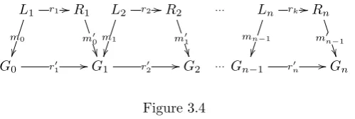
As mentioned before, the pushout construction can be used to apply a rule via a given match. We call the transformation of a graphGto a graphH using a rule p:L−→r R and a matchm:L→Ga direct transformation.

Definition 2.3.8 (Transformation). Given a rule p= L−→r R and a match

m: L→Gforp, thedirect transformation from Gwith rulepand matchm, written G =p,m⇒ H, is the pushout over r and m in GraphP_{. A sequence of} direct transformations of the form % = (G0

p1,m1

=⇒ . . . p=k,m⇒k Gk) constitutes a

transformation from G0 to Gk byp1. . . pk, abbreviated toG0

∗

=⇒Gk. Given

a set of rulesP, we say that a transformation G0

∗

=⇒Gk isterminating when

there is no rule in P that can be applied toGk.

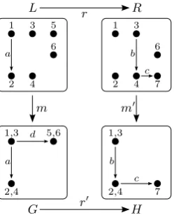
Example 2.3.9. Figure 2.1 shows an example of a direct transformation. We will explain how H was constructed by following Construction 2.3.4. In this explanation we name edges and vertices by the numbers written next to them. To avoid ambiguity, we will explicitly state in which graph the vertex or edge is. For example by (1,3)∈G we mean the top left vertex inG.

The first step of our construction is to define the relation∼as follows:

(1,3)∈G∼1∈R

(1,3)∈G∼3∈R

(2,4)∈G∼2∈R

(2,4)∈G∼4∈R

(5,6)∈G∼6∈R

Using∼we can form the following equivalence classes:

[(1,3)∈G] = [1∈R] = [3∈R] ={(1,3)∈G,1∈R,3∈R} = (1,3)∈H

[(2,4)∈G] = [2∈R] = [4∈R] ={(2,4)∈G,2∈R,4∈R} = (2,4)∈H

[(5,6)∈G] = [6∈R] ={(5,6)∈G,6∈R}

[7∈R] ={7∈R} = 7∈H

[a∈G] ={a∈G}

[b∈R] ={b∈R}

[c∈R] ={c∈R}

[d∈G] ={d∈G}

The set of verticesVHdoes not contain{(5,6)∈G,6∈R}, this is because the vertex

5∈L has no image underr, which means thatm(5∈L) = (5,6)∈G is deleted.

(23)

L

G H

R

1 3

a

2 4

5

6

1 3

2 4

6

7

b c

1,3

a

2,4 5,6

d 1,3

b

2,4 7

c

r0 r

m m0

Figure 2.1: Direct transformation by pushout. All edges have the empty label, the small letters (a-d) and the numbers show how vertices and edges are mapped under the morphismsr,r0,mandm0.

We can see thatr0_V((5,6)∈G) andm

0

V(6∈R) are both undefined since [(5,6)∈G] = [6∈R] and [6∈R]∈/ H. All other vertices in GandRhave an image under r0 or

m0_.

Now we construct the sets of edges, note that all edges have the empty label .

EH,add ={([(1,3)∈G], ,[(5,6)∈G]), ([3∈R], ,[4∈R])}

EH,del ={([3∈R], ,[4∈R])}

EH,all ={([3∈R], ,[4∈R]), ([4∈R], ,[7∈R])}

EH ={([3∈R], ,[4∈R]), ([4∈R], ,[7∈R])}

The edged∈Ghas no image underr0, this edge would be transformed to the edge

([(1,3)∈G], ,[(5,6)∈G]), which is in the setEH,add, however [(5,6)∈G]∈/VH(i.e.,

the edge has no target inVH), therefore the edge is not an element ofEH,all and

also not an element of EH. We also have rE0 (a∈G) undefined, because a∈G =

((1,3)∈G, ,(2,4)∈G), and ([(1,3)∈G], ,[(2,4)∈G]) = ([3∈R], ,[4∈R]) ∈ EH,del,

and d∈G ∈m(L) therefore, by construction of the edge morphisms rE0 (a∈G) is

undefined.

2.4

Single-Pushout High-Level Replacement

Sys-tems

In this section we present high-level replacement (HLR) systems using Single-Pushout, we consider a categoryC with a morphism classesRandM, where all morphisms inRare allowed as rule morphisms and all morphisms inMare allowed as matches.

(24)

Our definition for an SPO category differs from the definition given by Ehrig and L¨owe [14] in several ways. For example, [14] does not distinguish a class for morphisms which are allowed as rule morphisms, however for the transfor-mation of attributed graphs (see Chapter 5) we do need a separate class of rule morphisms to ensure that pushouts exist. The reason why our definition of an SPO category is different from the definition stated in [14] is because Ehrig and L¨owe use SPO categories to prove parallelism properties; we have not include the requirements for those parallelism properties in this definition.

Definition 2.4.1(SPO Category). LetC be a category with morphism classes MandR, then we call (C,M,R) anSPO category if the following properties hold:

1. C has pushouts over any morphism spanB ←−f A−→g C, if f ∈ Mand

g∈ R(or vice versa)

2. M and R are closed under composition, i.e., f : A → B ∈ M and

g:B→C∈ Mimpliesg◦f ∈ M(and the same forR)

3. M and R are closed under decomposition, i.e., g◦f ∈ M and g ∈ M impliesf ∈ M

The property 1 is needed to ensure that the pushout over a rule morphism and a match morphism always exists. Properties 2 and 3 are required for various proofs in the next chapters.

Proposition 2.4.2. Let M be the class of all total GraphP_{-morphisms, and} letRbe the class of all GraphP_{-morphisms, then} ₍_GraphP_,_M_,_R)_{is an SPO} category4_.

Proof. We prove every property of SPO categories separately:

1. GraphP _{has pushout over all morphisms}4_{, see Proposition 2.3.5}

2. The composition property follows from Definitions 2.1.2 and 2.1.3.

3. EveryGraphP_{-morphism is an}_{R-morphism, therefore the decomposition} property holds for R-morphisms. Let g◦f :A →C ∈ M, assume that

f /∈ Mleta∈Asuch that f(a) =⊥, then we know that (g◦f)(a) =⊥, a contradiction, therefore we can conclude thatM-morphisms are closed under decomposition.

Now that we know what an SPO category is, we formally define SPO HLR systems.

Definition 2.4.3 (SPO HLR System). AnSPO HLR system for an SPO cat-egory (C,M,R) consists of a set of rulesP.

• Every rulep= (L−→r R) ∈P consists of anR-morphismr.

• An objectG can be directly transformed to an object H by a rule p= (L −→r R) if there is aM-morphismm: L→G(called a match for p), and a pushout (G r

0

−→ H m

0

←− R) of (r, m) in C. In this case we write

G=p,m⇒H.

(25)

(26)

(27)

Chapter 3

Confluence, Conflicts,

Critical Pairs

In this chapter we will investigate sufficient conditions to decide if an HLR system is locally confluent. Before doing so, we will recall the relevant (general) notions of confluence, local confluence and termination.

We call a pair of transformationsX =∗⇒Y1,X

∗

=⇒Y2confluent when there exist transformations Y1

∗

=⇒ Z and Y2

∗

=⇒ Z. In other words, two diverging transformations are confluent when they can be joined again. An HLR system is called confluent if all derivable transformations are confluent.

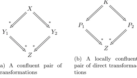
A weaker version of confluence is called local confluence, which essentially restricts confluence to direct transformations. A confluent pair of transforma-tionsK=∗⇒P1,K=∗⇒P2is calledlocally confluent when both transformations are direct transformations i.e., K =⇒ P1, K =⇒P2. The difference between confluence and local confluence is illustrated in Figure 3.1.

X

∗

z

∗$

Y1

∗

$

Y2

∗

z

Z

(a) A confluent pair of transformations

K

z

$

P1

∗

$

P2

∗

z

Z

(b) A locally confluent pair of direct transforma-tions

Figure 3.1: Confluence versus local confluence

We call an HLR system locally confluent when all pairs of direct transfor-mations in the HLR system are locally confluent. Local confluence of an HLR system alone does not imply confluence of the HLR system, the next example demonstrates this.

(28)

G0 +3

e0

G1 +3

e1

G2

e2

X0 +3X1 +3X2

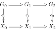
Figure 3.2: An embedding of%= (G0=⇒G1=⇒G2) intoδ= (X0=⇒X1=⇒

X2)

different direct transformations.

Aks B _b_j "*C +3D

There are two pairs of diverging direct transformations A ⇐= B =⇒ C and

B ⇐= C =⇒ D. We can reason that both pairs are confluent: A⇐=B =⇒

C is confluent because there exists a transformation C =∗⇒ A and similarly

B ⇐=C =⇒ D is confluent because there exists a transformation B =∗⇒ D. Since all pairs of direct transformations are confluent, we can conclude that the HLR system is locally confluent. As a whole, however, the HLR system is not confluent: for instance, the diverging pair of transformationsA⇐∗=C=⇒D is not confluent because bothAandD cannot be transformed any more.

We call a transformation X =∗⇒ Y terminating if no rules (in the HLR system) can be applied toY. An HLR system is terminating when there exist no infinite transformation sequences. An HLR system that is both locally confluent and terminating is also confluent [8].

For a locally confluent and terminating HLR system, all pairs of terminating transformation sequences X =∗⇒Y1 and X

∗

=⇒Y2 from the same start object, have targets equal up to isomorphism, i.e., Y1∼=Y2.

Confluence and local confluence of an HLR system is undecidable; however, in this chapter we provide sufficient conditions for establishing that an HLR system is locally confluent.

In order to prove our local confluence theorem we make use of so-called em-beddings. An embedding shows that a transformation%is contained (embedded) in another transformationδ, this means that for every (intermediate) objectGi

in %there exists an occurrence (M-morphism) to the (intermediate) objectXi

in δ (see Figure 3.2). Embeddings are used to show that the sequence of rules that are applied in the transformation % are applied in the transformation δ, and that the applications have the same effect.

In Section 3.1 we will formally define embeddings, and show when an em-bedding exists. We will need these emem-beddings later to prove our sufficient condition for local confluence of an HLR system. Section 3.2 will define what conflicts and critical pairs are, and we will prove that critical pairs are complete (in a sense defined below). In Section 3.3 we will investigate sufficient conditions to decide if an SPO HLR system is locally confluent, based on analysis of the critical pairs.

3.1

Embedding of Transformations

(29)

(30)

(31)

(32)

Proposition 3.1.8. Let r :L → R andm : L →G be GraphP_-morphisms, such that m ∈ M, where M is the class of total graph morphisms. Then r

is M-preserving w.r.t. m if and only m(x) = m(y) implies x, y ∈ dom(r) or

x, y /∈dom(r)1_.

Proof. The proof can be found in Appendix A.1

Next we define a more strict version of M-preserving morphisms, which states that every prefix (x1 is a prefix ofy of there exists a morphismx2 such that x2◦x1=y) of a strictlyM-preserving morphism (w.r.t. some morphism

x), must beM-preserving (w.r.t.x) as well.

Definition 3.1.9(StrictlyM-Preserving Morphism). LetC be a category with a classMof morphisms. Letm:A→B be aM-morphism and letf :A→C

be any morphism. We say thatf is strictlyM-preserving w.r.t.mif for every pair of morphismsf1, f2such thatf2◦f1=f, f1 isM-preserving w.r.t.m.

From the definition it follows that iff is strictlyM-preserving w.r.t.m, then

f is M-preserving w.r.t.m (takef1=f andf2 =idC). The next proposition

shows a direct consequence of the definition we have just given.

Proposition 3.1.10. Let C be a category with a classM of morphisms. Let

m :A→B be aM-morphism and let f :A →C be any morphism such that

f is strictlyM-preservingw.r.t. m, and letx1 andx2 be morphisms such that

x2◦x1=f, thenx1 is strictlyM-preservingw.r.t.m.

Proof. We know that x1 is strictly M-preserving w.r.t. m if for every pair or morphisms y1, y2 with y2◦y1 = x1, y1 is M-preserving w.r.t. m. We have

x2◦y2◦y1=f. Letf2=x2◦y2 andf1=y1, thenf1 isM-preserving w.r.t.m becausef is strictly M-preserving w.r.t.m.

We show a sufficient condition for when aGraphP _{morphism is strictly} M-preserving w.r.t. some morphism r. For M, we take the class of total graph morphisms.

Proposition 3.1.11. Let r:L →R andm:L→G beGraphP_-morphisms, such that m∈ M, whereM is the class of total graph morphisms. Then r is strictlyM-preservingw.r.t.mifm(x) =m(y)impliesx=y orx, y∈dom(r)1_.

Proof. Letm be a total morphism and r a morphism such that m(x) =m(y) impliesx=yorx, y∈dom(r). Letr1andr2be morphisms such thatr2◦r1=r. We must show that r1 is M-preserving w.r.t. m i.e. (by Proposition 3.1.8)

m(x) =m(y) impliesx, y∈dom(r1) orx, y /∈dom(r1). Assume to the contrary thatr1is notM-preserving w.r.t.m, i.e., there existx, y∈Lsuch thatm(x) =

m(y),x∈dom(r1) and y /∈dom(r1). This means thatx6=y andy /∈dom(r), which contradicts our conditions onr.

We can now answer the main question of this section: under which conditions can we embed a transformation into a different context. Ehrig et al. [13] have already given a similar proof (in the context of graphs) for embeddings where every morphism in the embedding must be injective (i.e., a monomorphism),

(33)

(34)

(35)

(36)

(37)

(38)

(39)

(40)

(41)

Chapter 4

Negative Application

Conditions

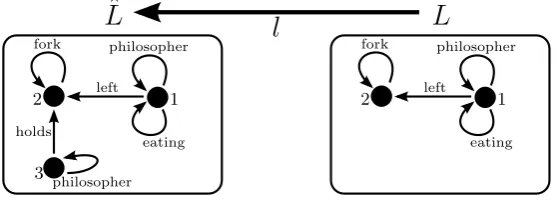
Up to this point we have considered HLR systems where the rules only consisted of a rule morphism. In this chapter we introduce rules withnegative application conditions (NACs). With NACs it is possible to specify when a rule may not be applied. In Figure 4.1 we see an graph Land a NACl :L→Lˆ. Assuming that L is the left-hand side of some rule pthen a match m : L →G for p is applicableonly if there does not exist a morphismn: ˆL→Gsuch thatn◦l=m; informally, the structure of ˆL must not exist inG.

We call an SPO HLR system where rules are allowed to have NACs anSPO HLR system with NACs.

ˆ

L

l

L

1

eating philosopher

left fork

2

3

2 1

eating philosopher

left fork

philosopher holds

Figure 4.1: ˆLis a NAC over L

(42)

4.1

Rules with NACs

In this section we will introduce (rules with) NACs, and we will prove some basic properties of NACs. We will start with a formal definition of NACs and rules with NACs.

Definition 4.1.1 (Negative Application Conditions). Given an SPO category (C,M,R) and a rule pwith rule morphismr:L→Rwe define the following:

1. Anegative application condition(NAC) overL(resp.R) is anR-morphism

l:L→Lˆ (resp.l0:R→Rˆ). We calll (resp.l0) aleft (resp.right) NAC onp.

2. An M-morphism m : L → X satisfies a left NAC l : L → _Lˆ_{, written}

m|=l, if there is noM-morphismn: ˆL→X such thatn◦l=m.

3. An M-morphismm :L →X satisfies a right NAC l0 : R →Rˆ, written

m|=l0, if, given the pushout X r

0

−→Y m

0

←−Roverr andm, if there is no M-morphismn: ˆR→Y such that n◦l0 =m0.

4. A (left or right) NACl:L→Lˆisfalsifiableif there exists anM-morphism

m: ˆL→X such thatm6|=l.

5. A (left or right) NACl:L→Lˆ isconsistent (or satisfiable) if there exists anM-morphismm:L→X such thatm|=l.

6. A rule with negative application conditions p= (L −→r R, A, B), or rule for short, consists of an R-morphism r, a set A of NACs over L (left NACs) and a setB of NACS overR(right NACs).

7. Given a rule with NACsp= (L−→r R, A, B), anM-morphismm:L→X

satisfies a setA(resp.B) of NACs, writtenm|=A(resp.m|=B) , if m

satisfies all NACs inA (resp.B) .

8. Given a rule with NACs p= (L −→r R, A, B), we say thatpisapplicable to an objectX at m : L→ X (written m|=p) if m∈ M, m |=A and

m|=B.

Letp= (L −→r R, A, B) be a rule and letl∈Abe a NAC forp. Ifl is not falsifiable (i.e., every match mforpsatisfies the NACl), then this means that the rulep0 _{= (}_L_−→r _{R, A}_{\ {}_l_}_{, B}_{) is applicable in the exact same situations as}

p. In the next proposition we will show when a left NAC is falsifiable.

Proposition 4.1.2 (Falsifiability of Left NACs). Let (C,M,R) be an SPO category; given a rule p = (L −→r R, A, B), a left NAC l : L → Lˆ ∈ A is falsifiable if and only ifl∈ M.

Proof. (⇒) Let l be falsifiable, then there exist M-morphisms m : ˆL → X

and n : ˆL → X such that n◦l = m. Since M-morphisms are closed under decomposition we can conclude thatl∈ M.

(43)

Remark. This does not hold for right NACs: given a rule p= (L −→r R, A, B) and an M-morphismm:L→Gthen given the pushoutX r

0

−→Y m

0

←−R over

randm, the morphismm0 may not be anM-morphism.

If a NACl is not falsifiable, then it does not add anything to the rule, since the same rule without the NACl is applicable in exactly the same situations. From this point we will assume that every left NAC is falsifiable, which means that every left NACl is both anR- and anM-morphism.

The next proposition states exactly when a NAC is consistent.

Proposition 4.1.3(Consistency of NACs). A (left or right) NACl:L→Lˆ is consistent if and only if there does not exist an M-morphism n: ˆL→L such that n◦l=idL.

Remark. Given morphismsl:L→Lˆ andn: ˆL→Lsuch thatn◦l=idL, then

we say thatnis a left inverse (or retraction) ofl.

Our proof is based on a similar proof in [13].

Proof. (⇐) If there does not exist anM-morphismn: ˆL→Lsuch thatn◦l= idL, thenidL|=l, i.e.,l is consistent by Definition 4.1.1.

(⇒) Letn: ˆL→Lbe anM-morphism such thatn◦l=idL. Since for any

given morphismm:L→Xwe havem=m◦idL, this implies thatm◦n◦l=m,

i.e.,m does not satisfy the NACl, thereforelis not consistent.

4.2

Converting Right NACs to Left NACs

Given a match m for a rule p = (L −→r R, A, B), then deciding if the match satisfies all left NACs is easier than deciding if the match satisfies all right NACs. This is because for right NACs we need to compute the transformation (i.e., the pushout over mandr) before we can decide if the match satisfies the right NACs.

If there would exist a rulep0 = (L−→r R, A0,∅) with the same rule morphism

r, which has only left NACs, such that for any M-morphism m : L →X we havem|=piffm|=p0 then it would be much easier to decide whether a rule is applicable. In this section we will investigate if there exists an equivalent rulep0

(without right NACs) for any rulepsuch thatpandp0are applicable in exactly the same situations.

One way to find such an equivalent rule, is to convert every right NAC into a number of left NACs. Consider a rule p= (L −→r R, A, B), whereB is non-empty. Then we want to find a set of left NACsA0 ₌_{_l

1:L→Lˆ1, . . . , ln→Lˆn}

such that for every M-morphismmwe havem|=A0 if and only ifm|=p. To construct the setA0 we will usepushout complements.

Definition 4.2.1 (Pushout Complement). Given morphisms f : A → B and

h : B → D, a pushout complement of (f, h) is an object C and morphisms

g:A→C andi:C→D such that the cospan C−→i D ←−h B is the pushout over f and g. Two pushout complements Cj with morphisms gj : A → Cj

and ij :Cj →D forj = 1,2 are isomorphic when there exists an isomorphism

(44)

(45)

(46)

(47)

In the next section, most of our proofs will require that the NAC equivalence property holds. Proving that this property holds for (GraphP_,_M_,_{R) is future} work.

4.3

Derived Rules and Embeddings

In this section we will formulate a new embedding theorem which allows rules with NACs. In order to be able to do so we will define derived rules. Similarly to transformation morphisms (as defined in Definition 3.1.3), a derived rule is derived from a transformation. In fact, the rule morphism of a derived rule is the transformation morphism of the transformation. A derived rule also has a set of left NACs, which we will explain in more detail at a later point.

First we will define another assumption that we must make, namely that the SPO category that we use is closed under pushouts over M-morphisms. The meaning of this is defined below.

Definition 4.3.1. Given an SPO category (C,M,R), we say that M-mor-phisms are closed under pushouts if for anyf :A→B ∈ M,g:A→C ∈ M andg∈ R(gis both anM- and anR-morphism) then the pushout over (f, g) is also a pushout in the category with the same class of objects asC and the class ofM-morphisms1_.

Proposition 4.3.2. In the SPO category(GraphP_,_M_,_R),_{M-morphisms are} closed under pushouts.

Proof. M-morphisms are total graph morphisms. We can use Construction 2.3.4 1_{to construct the pushout of two total graph morphisms, we can repeat the proof}

of Proposition 2.3.5 to show that pushouts exist in the category with the object class of all graphs and morphisms in the classM.

Next we will define derived rules. First we will define a so-called single-step derived rule. This is a rule (with a set of NACs), which is derived from a single-step transformation.

Definition 4.3.3 (Single-Step Derived Rule with NACs). Given an SPO cate-gory (C,M,R) whereMis closed under pushouts. Let p= (L −→r R, A) be a rule whereA={l1, . . . , ln} and let%= (X

m,p

=⇒Y) be a transformation. The

single-step derived rule ¯%= (X −→%ˆ Y, A0) of%is defined as follows: • %ˆis the transformation morphism of%;

• A0 = {l0₁, . . . , l0_n} such that, fori = 1. . . n, l0_i is the co-morphism of li :

L→Lˆi in the pushout ˆLi

ˆ

m0

i −→Xˆi

l0_i

←−X overm andli.

Remark. We know that everyl0_i∈Ais anM-morphism becauseM-morphisms are closed under pushouts.

Next we will show that the definition we have just given is correct, in the sense that the NACs for the derived rule are satisfied under precisely the right circumstances.

(48)

(49)

(50)

M-preserving w.r.t.e0 (by Proposition 3.1.10) and we also know thate0 |= ¯% because of Lemma 4.3.6.

Because we havee0 |= ¯% we can apply the induction step. The rest of the proof (including the base case for the induction, where we do not have any NACs at all) is analogous to Theorem 3.1.12.

4.4

Critical Pairs and Confluence

In Section 3.3 we have seen that the embedding theorem is important for proving that an HLR system (without NACs) is strictly locally confluent if all critical pairs are strictly locally confluent.

Given a transformation % = (G0

∗

=⇒ Gn) and an M-monomorphism e0 :

G0 → X0, all conditions of the original embedding theorem (Theorem 3.1.12) are satisfied (because all R-morphisms are strictly M-preserving w.r.t. any monomorphism in M). We cannot say the same for our new embedding theo-rem, since the fact that e0 is a monomorphism does not necessarily mean that

e0 satisfies all NACs of the derived rule ¯%. Because of this, finding a sufficient condition for strict local confluence for HLR systems with NACs is not easy.

In this section we will define parallel independence for transformations with NACs. We will define critical pairs with NACs. We will also show that it is not easy to prove strict local confluence of an HLR system based on analysis of the critical pairs, since critical pairs do not only depend on a pair of transformations, but they should take other rules in the HLR system into account.

Definition 4.4.1 (Parallel Independence). Let t1 = (X

p1,m1

=⇒ Y1) and t2 = (X p2,m2

=⇒ Y2) be two direct transformations using p1 = (L1

r1

−→ R1, A1) and

p2= (L2

r2

−→R2, A2). Thent1 andt2are parallel independent ifm∗1=r02◦m1 is a match for p1, and m∗₂ = r0₁◦m2 is a match for p2 with m∗1 |= p1 and

m∗₂ |=p2. We call a pair of transformationsparallel dependent, if they are not parallel independent.

From this definition we can see that there can be different reasons why a pair of transformations is parallel dependent. First of all, it can be the case that m∗1=r20 ◦m1is not a match forp1, or m∗2=r10 ◦m2 is not a match forp2 (i.e.,m∗

1∈ M/ orm∗2∈ M). This is a/ delete-use conflict, which we have already seen in Section 3.2 on page 31. The other reason why a pair of transformations can be parallel dependent is the situation wherem∗₁ 6|=p1 orm∗2 6|=p2. Such a situation is called a produce-forbid conflict, since one rule produces something which is forbidden by one of the NACs of the other rule.

It is possible that a parallel dependent pair of transformations has both a delete-use conflict and a produce-forbid conflict, for instance if m∗₁ ∈ M/ and

m∗₂∈ Mbut m∗₂6|=p2.

Given the new definition for parallel independence, we can prove that all parallel independent pairs of transformations in a HLR system with NACs are strictly locally confluent.

Theorem 4.4.2(Strict Local Confluence of Parallel Independent Direct Trans-formations). Given an SPO HLR system with NACs, lett1= (G

p1,m1

(51)

(52)

(53)

(54)

(55)

Definition 4.4.8(Strict NAC-confluence). A conditional critical pair of trans-formations t1= (K

p1,m1

=⇒ C1) and t2 = (K

p2,m2

=⇒ C2) is strictly NAC-confluent if

1. it is strictly confluent via some transformations%1= (K

p1,m1 =⇒ C1

∗

=⇒X) and%2= (K

p2,m2 =⇒ C2

∗

=⇒X)

2. and for every morphism e0 : K → G ∈ M where e0 |= ¯t1 and e0 |= ¯t2 (i.e.,e0satisfies the derived rules oft1andt2), it follows thate0|= ¯%1and

e0|= ¯%2(i.e.,e0 satisfies the derived rules of%1and%2).

Using this definition, we would be able to prove that an SPO HLR system is strictly locally confluent if all conditional critical pairs are strictly confluent (this proof would be analogous to Theorem 3.3.4, the strict NAC-confluence ensures that the embedding theorem with NACs is applicable).

What we do not yet know is when a conditional critical pair is strictly NAC-confluent. Lambers [23] provides a sufficient condition for strict NAC-confluence in the DPO setting, it should be investigated if these conditions also work for in the SPO setting.

(56)

(57)

Chapter 5

Attributed Graphs

In this chapter we will introduce attributed graphs and show that attributed graphs can be used for SPO high-level replacement. Attributed graphs are graphs where some vertices represent values, such as integers, strings, booleans or characters. These value vertices may only be the target of edges.

In Figure 5.1 we see an example of a rule with uses attributed graphs. In the rule the vertex labelled 1 in the attributed graph L represents a hungry philosopher. The edge ‘forks’ points to a vertex with the integer value 2, which means that the philosopher has two forks. This rule removes the edge with the label ‘hungry’, and adds a self edge with the label ‘eating’.

L

r

R

1

2

hungry philosopher

forks

1

2

eating philosopher

forks

Figure 5.1: A rule which transforms a hungry philosopher with two forks to an eating philosopher with two forks.

In the graphsL andR we have shown only one value vertex. However, for every integer there exists a unique value vertex in both graphs L and R; we only display those value vertices which have incident edges.

In Section 5.1 we will introduce algebraic signatures and algebras, which are necessary to define attributed graphs. In Section 5.2 we will define attributed graphs and show that there exists an SPO category with attributed graphs as objects.

5.1