Using a Goal-Switching Selection Operator in Multi-Objective Genetic Algorithm Optimization Problems.

(1)

ABSTRACT

SHAEFER, DANIEL MARK. Using a Goal-Switching Selection Operator in Multi-Objective Genetic Algorithm Optimization Problems. (Under the direction of Dr. Scott Ferguson).

(2)

(3)

Using a Goal-Switching Selection Operator in Multi-Objective Genetic Algorithm Optimization Problems

by

Daniel Mark Shaefer

A thesis submitted to the Graduate Faculty of North Carolina State University

in partial fulfillment of the requirements for the degree of

Master of Science

Aerospace Engineering

Raleigh, North Carolina 2013

APPROVED BY:

_______________________________ ______________________________ Dr. Hong Luo Dr. Lawrence Silverberg

________________________________ Dr. Scott Ferguson

(4)

DEDICATION

(5)

BIOGRAPHY

Daniel received his BS in Aerospace Engineering from North Carolina State University in 2011. While an undergrad, he was active in the school’s Aerial Robotics club and served as Vice President from 2009-2010. It was that year that NCSU ARC won first place in the flight testing phase and the overall combined score. For his senior design, he designed, built, and saw his canard plane with reconfigurable wings fly at Perkins Field in Butner, NC. He worked on the performance and aerodynamics for the plane, spending many late nights working on CMARC.

(6)

ACKNOWLEDGMENTS

(7)

TABLE OF CONTENTS

LIST OF TABLES ... viii

LIST OF FIGURES ... ix

1. INTRODUCTION... 1

1.1 Optimization in Engineering Design ... 1

1.2 Defining the Pareto Frontier ... 1

1.3 Solving for the Pareto Frontier ... 3

1.3.1 Weighted Sum ... 3

1.3.2 Particle Swarm ... 4

1.3.3 Evolutionary Algorithms ... 5

1.4 Design by Shopping ... 8

1.5 Research Questions ... 9

1.5.1 Research Question #1 ... 11

1.5.2 Research Question #2 ... 12

1.6 Thesis Organization... 12

2. BACKGROUND ... 14

2.1 Overview of Multi-Objective Genetic Algorithms ... 14

2.2 Population Creation ... 15

2.3 Selection ... 16

2.4 Crossover ... 18

2.5 Mutation ... 19

2.6 Insights from the Literature Review... 20

3. Development of the Goal Switching Method ... 22

3.1 Concept of Goal Switching ... 22

3.2 General Methodology ... 23

3.2.1 Define Algorithm Goals ... 24

3.2.2 Establish Switching Index... 25

3.2.3 Define Switching Order ... 25

3.2.4 Choose Selection Percentage ... 26

3.2.5 Select Selection Operator ... 26

(8)

3.3.1 Define the Problem ... 27

3.3.2 Define the Assessment Metrics ... 28

3.3.3 Define Parameters for Selection Operator with Goal Switching ... 30

3.3.4 Run the MOGA with Default Selection Operator... 31

3.3.5 Run the MOGA with Updated Selection Operator ... 32

3.3.6 Compare Results ... 33

3.4 Chapter Summary ... 38

4. GOAL SWITCHING PARAMETER ANALYSIS ... 39

4.1 Introduction ... 39

4.1.1 Design of Experiments Analysis ... 40

4.1.2 Main Effects and Linear Model Fit ... 43

4.2 CASE STUDY 1 – MP3 Player Product Line Design Problem ... 46

4.3 CASE STUDY 2 – Two Bar Truss Design ... 70

5. CONCLUSIONS AND FUTURE WORK ... 92

5.1 Thesis Summary... 92

5.2 Addressing the Research Questions ... 94

5.2.1 Research Question 1 ... 94

5.2.2 Research Question 2 ... 96

(9)

(10)

LIST OF TABLES

Table 3.1 UF1, 50%, 10,000 Evaluations, SI=5 ... 32

Table 3.2. UF1, 50%, 10,000 Evaluations, SI=5 ... 33

Table 3.3. UF1, 4 DVs, 10,000 Evaluations, SI=5 ... 36

Table 4.1. Goal Switching Design of Experiments Layout ... 39

Table 4.2. Analysis of Variance Data Layout ... 41

Table 4.3. Example Mapping Relationship between Index Number ... 44

Table 4.4. Example Linear Model Fit Data Layout ... 46

Table 4.5. MP3 Player Attributes and Price Levels ... 47

Table 4.6. MP3 Player Cost Per Feature ... 50

Table 4.7. Design of Experiments MP3 Reference ... 51

Table 4.8. Baseline Results, MP3 Problem... 53

Table 4.9. MP3 Roulette Selection Analysis of Variance Results ... 54

Table 4.10. MP3 Roulette Selection Linear Fit Results... 55

Table 4.11. MP3 Main Effects Plot Summarized Results, Roulette Selection ... 58

Table 4.12. MP3 Tournament Selection Analysis of Variance Results ... 59

Table 4.13. MP3 Tournament Selection Linear Fit Results... 60

Table 4.14. Main Effects Plot Summary Tournament MP3 ... 63

Table 4.15. MP3 Roulette Mean Analysis ... 64

Table 4.16. MP3 Roulette Nested Analysis ... 65

Table 4.17. MP3 Tournament Mean Analysis ... 65

Table 4.18. MP3 Tournament Nested Analysis ... 66

Table 4.19. Design of Experiments Two Bar Reference ... 73

Table 4.20. Two Bar Roulette Selection Analysis of Variance Results ... 75

Table 4.21. Two Bar Roulette Selection Linear Fit Results ... 77

Table 4.22. Main Effects Plot Summary Roulette Two Bar ... 80

Table 4.23. Two Bar Tournament Selection Analysis of Variance Results ... 81

Table 4.24. Two Bar Tournament Selection Linear Fit Results ... 82

Table 4.25. Main Effects Plot Summary Tournament Two Bar ... 85

Table 4.26. Two Bar Truss Roulette Mean Analysis ... 86

Table 4.27. Two Bar Truss Roulette Nested Analysis ... 87

Table 4.28. Two Bar Truss Tournament Mean Analysis ... 88

Table 4.29. Two Bar Truss Tournament Nested Analysis ... 88

Table 5.1. Roulette Adaptive Goal Switching Results ... 100

(11)

LIST OF FIGURES

Figure 1.1. Pareto Optimal Example [3] ... 3

Figure 1.2. Pareto Frontier Ranking [13] ... 7

Figure 3.1. Goal Switching Analogy Visualization ... 23

Figure 3.2. Factors Defined when Constructing the Selection Operator ... 24

Figure 3.3. Pareto Frontier of UF1... 28

Figure 3.4. Boundary Points Added for Hypervolume Calculation... 30

Figure 3.5. Convergence of Goal Switching and Roulette on UF1 for 3 DVs, 50% ... 34

Figure 4.1. Example Main Effects Plot ... 44

Figure 4.2. MP3 Hypervolume Main Effects Plot, Roulette Selection ... 56

Figure 4.3. MP3 Crowding Distance Main Effects Plot, Roulette Selection ... 56

Figure 4.4. MP3 Frontier Points Main Effects Plot, Roulette Selection ... 57

Figure 4.5. MP3 Hypervolume Main Effects Plot, Tournament Selection ... 61

Figure 4.6. MP3 Crowding Distance Main Effects Plot, Tournament Selection ... 61

Figure 4.7. MP3 Frontier Points Main Effects Plot, Tournament Selection ... 62

Figure 4.8. Pareto Frontier for (f1, f2) Switching Mode (L) and (f1, f2, both) Switching Mode (R), 25% Selection ... 69

Figure 4.9. Pareto Frontier for (f1, f2) Switching Mode (L) and (f1, f2, both) Switching Mode (R), 50% Selection ... 69

Figure 4.10. Pareto Frontier for (f1, f2) Switching Mode (L) and (f1, f2, both) Switching Mode (R), 75% Selection ... 70

Figure 4.11. Two Bar Truss Diagram ... 71

Figure 4.12. Two Bar Hypervolume Roulette Main Effects Plot ... 78

Figure 4.13. Two Bar Crowding Distance Roulette Main Effects Plot ... 78

Figure 4.14. Two Bar Frontier Points Roulette Main Effects Plot ... 79

Figure 4.15. Two Bar Hypervolume Tournament Main Effects Plot ... 83

Figure 4.16. Two Bar Crowding Distance Tournament Main Effects Plot ... 83

(12)

1. INTRODUCTION

1.1 Optimization in Engineering Design

Optimization is used in many engineering disciplines and scientific fields to improve a performance measure or provide insight into a forthcoming decision [1]. In aeronautical engineering specifically, optimization can be especially helpful in the embodiment and detailed design phases. The goal in embodiment design is to explore the design space in an effort to improve performance while managing the tradeoffs present when multiple objectives and multiple disciplines are considered [2]. Multi-objective optimization problems (MOPs) are characterized by the competing nature of the simultaneously considered performance parameters. Solutions to multi-objective problems exist as a set of solutions, as opposed to the single design vector common to single objective formulations. A unique property of this set of solutions is that each individual design in the set does not dominate, or is not dominated by, the other designs. Locating this set of solutions in the most effective and efficient manner possible is a fundamental research challenge in the area of engineering optimization.

1.2 Defining the Pareto Frontier

(13)

as Pareto points. This set of Pareto optimal points is called a Pareto frontier. A Pareto

dominant solution is one with a feasible design variable vector, x', for which there is no

other feasible design variable vector, x, which meets the following criteria, )

' ( ) (x f x

f_i ≤ _i for i = 1,n

) ' x ( f ) x (

f_i < _i for at least one i, 1 ≤ i ≤ n (1.1)

where n is the number of objective functions.

This concept is easily visualized in two-dimensional space. In Figure 1.1, the Pareto optimal points are shown in brown and the dominated points are in green. When choosing between brown points, Objective 1 can only be improved (assuming minimization of both objectives) if a decreased performance in Objective 2 is accepted. However, any green point can be improved in Objective 1 and / or Objective 2 by moving to a brown point.

(14)

Figure 1.1. Pareto Optimal Example [3]

1.3 Solving for the Pareto Frontier

There are a multiple approaches that can be used to generate Pareto frontiers for multi-objective optimization problems. A few examples include weighted sum, particle swarm, and evolutionary algorithms. Each of these listed algorithms will be explained below to provide a description of their general approach and to highlight strengths and weaknesses.

1.3.1 Weighted Sum

(15)

= ∑ ( ) (1.2) In this approach, the objective functions (Fi) are combined into a single function (U) using weighting terms, wi, to signify the contribution of each objective. Here, k is the number of objectives being optimized. A constraint on the weight terms is that each wi must be between 0 and 1, and that the sum of the weights is equal to 1. Since each weight combination generates a single solution, a set of points is found by running the optimization with multiple weighting schemes. However, as each weight scheme has to be optimized, the large number of evaluations associated with this process results in significant computational inefficiency.

Though simple to use, selecting an appropriate weight scheme is a significant challenge. Further, choosing a weighting scheme as a starting point and varying it methodically does not guarantee an even distribution of points along the frontier. This methodological variation is also incapable of finding points on the non-convex parts of the Pareto frontier [5–7].

1.3.2 Particle Swarm

(16)

PSO has been adapted to multiobjective optimization problems by evaluating one objective function at a time or by using algorithms to evaluate every objective for each particle [9,10]. Considering one objective at a time leads to an aggregation function similar to a weighted sum. This necessitates multiple optimization attempts with different weighting schemes to obtain the desired number of non-dominated solutions. When all objectives are considered, the algorithm must determine sets of particles that have non-dominated positions, and use those to guide the rest of the swarm. Choosing the non-dominated particles that should lead the swarm is challenging, however, since there can be many solutions that are non-dominated.

1.3.3 Evolutionary Algorithms

All evolutionary algorithms (EAs) are based on the idea of a population of solutions that undergo a reproduction process to generate new solutions. One specific implementation of Pareto-based EAs is an elitist algorithm called Nondominated Sorting Genetic Algorithm II (NSGA-II) [11], a variation on the non-elitist NSGA [12]. Genetic Algorithms (GAs) are attractive for engineering optimization problems because of their robustness and their relative simplicity. They are also easy to parallelize, easy to hybridize, and can generate a variety of solutions.

(17)

evolutionary process in plants and animals. That is, new offspring are a combination of their parents’ genetic material.

(18)

Figure 1.2. Pareto Frontier Ranking [13]

(19)

1.4 Design by Shopping

One approach for selecting points from the Pareto frontier is to implement a weighting scheme between objectives, aggregate performance and weighting information into a single score, and then take the best score as the final answer. Creating a weighting scheme requires a user to identify their options, develop expectations of each choice, and form a system of values to rank each outcome [14]. However, this method is dependent on the designer being able to assign weights to each objective correctly, as different weights can lead to different decisions [15]. Decisions about strength of preference curves and weighting schemes must also be done before the designer has information about the behaviors seen in the design and performance spaces.

(20)

The hyper-space diagonal counting (HSDC) method, for example, has been developed to show lossless mapping of multiple dimensions. The key idea behind this method is linking multiple objectives per index [20]. When using this method a four objective problem would have two objectives per axis. The Preference Range and Uncertainty Filtering (PRUF) method is an extension of this idea and uses hyper-radial visualization to visualize the multi-objective space [21]. This method integrates uncertainty so the designer can view the performance space under different preference conditions. Further, tools like the Applied Research Laboratory Trade Space Visualizer (ATSV) use a combination of real-time visualization and designer input to guide the optimization with the hope that a knowledgeable designer can help the optimization by manually pointing it in the right direction [22].

If the design-by-shopping concept is to be used, a designer must be presented with a solution set of feasible designs. Having the best information possible is important, as the designer can only make a decision based on the information they have available. If the Pareto frontier found by an optimization is incomplete, or is not an accurate representation of the true Pareto frontier, the designer will lack the information needed to make a correct assessment of the required tradeoffs. If the results from an optimization can be improved, the Pareto frontier will more closely resemble that of the true Pareto frontier, enabling the designer to make the most informed decision possible.

1.5 Research Questions

(21)

optimization is design steering, where a user actively interacts with the GA as it is running [22–26]. By viewing the Pareto frontier in real-time or near real-time, the user can observe the progress of the algorithm and can directly modify the behavior of the GA. One example approach is the placement of an attractor in the performance space that acts as a new optimum for the optimization problem. Here, solutions are given better scores as the distance to the attractor becomes smaller. Using this technique the user can try to fill gaps in the observed Pareto frontier or can focus in on areas that they deem to be important [23].

This thesis introduces a goal switching approach for multiobjective optimization that acts as a way of focusing on various parts of the Pareto frontier without active human intervention. Prior research completed on temporal goal switching [27] has shown periodically switching between related goals can improve solution quality. This research was directed toward weighted-sum single objective problem formulations, and extending this concept to multiobjective formulations is the motivation for this work.

The goal switching method introduced in this paper attempts to improve solution quality of Pareto frontier by creating an improved selection operator. It draws from the sub-population selection and the Pareto rank-based selection methods from NSGA-II, and uses the sharing function metric of crowding distance. This goal switching method attempts to accomplish the same task as an attractor-based method, minus the active human intervention. Further, the goal switching selection method is simple to implement in code and will not interfere with previous selection methods; it merely augments them.

(22)

in a higher quality Pareto frontier. The second question investigates the robustness of the goal switching method by studying the effects of changing the parameters that define the behavior of the method.

1.5.1 Research Question #1

What are the impacts on Pareto frontier solution quality when the

selection operator of a MOGA is modified to include goal switching?

Periodical temporal switching is an elegantly simple way of increasing design diversity with low computational overhead. It has been shown that MOGAs and temporal modifications to the crossover operator can be combined [28], so integrating this concept into the selection operator may lead to improved solution quality.

(23)

improvement in the overall quality of the Pareto frontier with minimal impact on the computational overhead associated with the selection operator.

1.5.2 Research Question #2

How does Pareto frontier solution quality change when parameters controlling goal

switching behavior are modified?

Integrating goal switching into the selection operator of a MOGA will likely lead to additional input parameters that influence final solution quality. This question explores the robustness of solution quality when goal switching is used by exploring algorithm sensitivity to these input parameters

1.6 Thesis Organization

(24)

(25)

2. BACKGROUND

2.1 Overview of Multi-Objective Genetic Algorithms

The versatility of multi-objective algorithms (MOAs) has allowed them to be applied by numerous disciplines to help solve complex optimization problems. To improve solution quality and reduce computational cost, every discipline tunes an MOA using its own algorithms and modifications. Additionally, there are a variety of different MOAs such as genetic algorithms (GAs) [11], particle swarm algorithms [30], and hybrid techniques [30,31]. Because of the simplicity, ease of use, and practicality towards multi-objective optimization, a subset of GAs called multi-objective genetic algorithms (MOGAs) are chosen to provide the base for the thesis research. Contained under the MOGA classification there is a large amount of diversity. NSGA-II has already been discussed, but there is also Niched Pareto Genetic Algorithm 2 (NPGA 2) [32] that uses tournament selection like the original NSGA, and Micro-Genetic Algorithm that partially reinitializes its population after every generation [33,34].

(26)

parents’ traits, which can be modified even further by the mutation technique. This process of selection, crossover, and mutation repeats until a solution or ending condition is met.

Each of these four operators have parameters that can be tuned, which can be a laborious task if users are forced to resort to tuning each parameter separately [35]. Changing one parameter can also affect the other parameters, and different settings can be beneficial for different stages of the optimization. However, general settings can sometimes be applied over a large range of problems [36].

The current state of the four GA operators will be examined over the course of this chapter, noting the different ways each technique can be used. The chapter ends by discussing how these works influence the goal switching concept developed in Chapter 3.

2.2 Population Creation

(27)

Because GAs evaluate many design during their execution, it can be computationally inefficient to store and access every design tested. It can be especially inefficient to compare each design to every other design as is done when performing Pareto-ranking. Size of the population is sometimes limited as an optimization progresses to conserve computer resources or speed up convergence. Small starting populations have been shown to be highly unreliable, especially in the absence of diversity maintaining operators such as mutation. Large populations can be useful on difficult problems if computation time is not a factor [43]. Further, the population size can be dynamically controlled by implementing techniques such as age, where after a finite amount of time the point is removed from the solution set [44]. A risk here is that, by purging results, it is possible to remove the best points because they have reached old age.

The main parameter being altered in the population creation step is the starting population size, while a secondary concern is how to handle the population as the optimization progresses. If the population is too small, the optimization might never reach the intended convergence. A population that is too large suffers a convergence time penalty.

2.3 Selection

(28)

such as Developed Back Controlled Selection Operators (BCSO) take existing selection operators and apply them to each member of the population. The concept of this approach is to take the current fitness value of a point and compare it to past values of itself [45].

Classification of the different types of selection operators has identified five categories: sub-population parallel selection, aggregation by variable objective weighting, Pareto rank-based selection, sharing function approach, and external population selection [48].

The population parallel method works by dividing the total population into populations of equal size by selecting for each objective individually. Each of these sub-populations progress independently and the winners of each group are combined for the remainder of the GA. Challenges with this method are that the sub-populations rely on the single objective problem they were solved for, and that solutions found tend to exist on the extremes of the Pareto frontier.

Aggregation by variable objective weighting gives each objective a weight and then calculates the fitness value by summing the weights. The advantage here is that the selection process can be done in parallel, so it is more efficient. Pareto rank-based selection scores designs based on their non-dominated rank, so designs that are non-dominated receive the lowest rank, and designs dominated by more designs receive a higher rank. This process can be slow and can create many similar designs.

(29)

calculating crowding distance. Finally, external population selection saves a secondary population of good results so they are not lost due to the randomness of the algorithm [48].

The main selection operator modification that is most similar to goal switching is VEGA [49], developed by Schaffer. This multi-objective algorithm modifies the selection operator so several sub-populations are generated for each generation. Sub populations are of size N/k, where ‘k’ is the number of objectives and ‘N’ is the total population size. Each sub-population is taken from a proportional selection from each objective in order and then they were combined. A limitation of this approach is the occurrence of speciation, where individuals perform well in one objective but are only average when all objectives are considered.

2.4 Crossover

(30)

optimizing a variety of engineering problems [54,55]. There are also more exotic versions of crossover, such as ring crossover, where parents are connected end to end and sliced randomly. One child inherits half of the characteristics travelling clockwise from the cut location, the other travelling counterclockwise. Results show that this method is slightly better than existing methods, by maintaining a better variety [56].

Crossover operators vary by the number of times they split a parent before combining information to form children. The combination order can also be varied to produce different types of crossover operators. Improving crossover techniques can be done by choosing or cycling through a variety of operators. By not relying on one operator technique to maintain diversity, the solutions can advance without becoming stuck in local minimums.

2.5 Mutation

(31)

so maintaining constant selection pressure by varying mutation throughout the optimization can prevent premature convergence [60].

This thought process is further motivation for incorporating goal switching into the selection operator. The constant switching of parameters maintains diversity in the population while continuing to progress the frontier. One of the best mutation switching algorithms is that of the Borg MOEA [61], which can handle problems with four or more objectives by using multiple search operators that adapt to problem landscapes. It also uses a restart mechanism if the program senses local convergence or search stagnation [62]. Varying the mutation parameters like mutation rate and mutation type are the main ways to alter the behavior of the optimization with the mutation operator, and only small changes in rate are needed to significantly impact results.

2.6 Insights from the Literature Review

The above literature review demonstrates that constantly varying parameters and algorithms results in better solutions. This lends credence to the hypothesis that goal switching selection will improve solution quality of the Pareto frontier. Further, periodical switching has been said to prevent speciation due to the random cycling of the optimization, so the added benefit from considering crowding distance and Pareto rank should allow goal switching to successfully improve Pareto frontier solution quality.

(32)

(33)

3. Development of the Goal Switching Method

3.1 Concept of Goal Switching

This thesis introduces how the selection operator of a MOGA can be modified through the addition of goal switching. Goal switching is a way of dynamically filtering the list of potential candidates before performing the act of selection - using techniques like roulette or tournament selection. Because goal switching only modifies the list of potential candidates, it can be incorporated into any selection operator without changing how the other MOGA operators behave. The goal of this thesis is to determine the extent by which the solution quality of a Pareto frontier can be improved relative to the results found using a baseline selection technique.

An analogy that helps visualize goal switching is a fire hose nozzle. If a fire hose is used without a nozzle, it sprays water in an unfocused manner. This can lead to gaps in the frontier and large clusters of points in other locations. By applying the analogous nozzle, goal switching can shift the behavior of the algorithm by concentrating on specific areas of the performance space. Flow can then be redirected to focus on a different area after a set time period has elapsed. It is hypothesized that switching back and forth between these “goals” will lead to improved solution quality.

(34)

selection operator can advance specific regions of the Pareto frontier. The green curve represents the new Pareto frontier at each time step.

Figure 3.1. Goal Switching Analogy Visualization

After a few goal switching operations, the entire Pareto frontier can be moved in a beneficial direction with little to no internal computational effort. However, the designer must decide where to direct the stream, how much focus it should have, and when the direction of the stream should be changed. Defining these parameters in the context of the goal switching algorithm is completed in the next section.

3.2 General Methodology

(35)

included. The following subsections describe the need for each factor and how the factor might influence Pareto frontier solution quality.

3.2.1 Define Algorithm Goals

The first step of this approach is to define the goals of the algorithm. By doing so, the foci of the selection operator are established. Defined goals can be in the form of a single objective, a subset of problem objectives, or the full set of problem objectives. A goal with fewer objectives will have a more directed search, while a goal characterized by multiple objectives will result in a broader search.

For example, in a two-objective optimization problem there are three possible goals that can be defined:

• Minimize F1 only

• Minimize F2 only

Select selection operator

Choose selection percentage

Define switching order

Establish switching index

Define algorithm goals

(36)

• Minimize F1 and F2

3.2.2 Establish Switching Index

Having defined the goals of the algorithm, the next step is to define the frequency by which the algorithm iterates between these goals. In this work, the switching index (SI) is used as the parameter that defines the duration under which a single goal is considered. A low value of the switching index indicates quick switching between goals. This will increase the diversity of the search – by essentially creating a high level of randomness – but may also prevent significant improvement in solution quality. A large SI value will allow for a more directed search, but may constrain improvement to a portion of the performance space depending on the active goal.

In this work, the switching index is defined using algorithm generations as the timer value. Other available options include number of function evaluations, computational run-time, and measures of frontier stagnation, for example.

3.2.3 Define Switching Order

(37)

3.2.4 Choose Selection Percentage

The selection percentage is a number greater than 0% and less than or equal to 100%. Here, 100% indicates the possibility of choosing points from the entire population. As this number gets closer to 0%, population points that perform the worst with respect to the active goal are removed from selection consideration. By selecting a low cut percentage, the edges of the Pareto frontier are advanced much more quickly than the middle of the frontier. This percentage value is effectively an additional filtering mechanism.

3.2.5 Select Selection Operator

Finally, the selection operator for the MOGA must be chosen. The goal switching aspect of this approach only orders and filters the designs that exist in the population. By itself, no designs are selected for crossover and mutation. Defining a selection operator – such as tournament or roulette – is necessary to build the vectors of parent designs that will be used to create offspring.

3.3 Testing the Selection Operator with Goal Switching

(38)

1) Define the problem

2) Define the assessment metrics

3) Define parameters for selection operator with goal switching 4) Run the MOGA with default selection operator

5) Run the MOGA with updated selection operator 6) Compare results

The following sub-sections explore the testing sequence using the UF1 problem from CEC 09 [63].

3.3.1 Define the Problem

The first step of this procedure is to fully define the problem. In this case, the problem has two objective functions to be minimized. As shown in Equation 3.1, n is the number of design variables, x1 is the first design variable, J1 = {j|j is odd and 2 ≤ ≤ }, J2 = {j|j is

even and 2 ≤ ≤ }, and j is the current design variable counter.

= +_{| |}2 − sin(6 + )

∈"#

(3.1)

= 1 − +_|2_| − sin(6 + )

∈"%

(39)

= 1 − & , 0 ≤ ≤ 1

(3.2)

= sin(6 + ) , = 2, … , , 0 ≤ ≤ 1

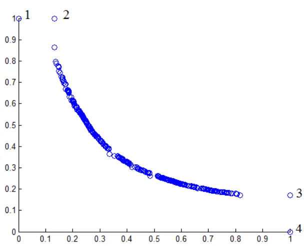
Figure 3.3. Pareto Frontier of UF1

Problems from CEC 09 were developed to be scalable to any amount of variables. For this problem, the number of design variables needs to be at least three. To explore the scalability of this approach, the problem is studied using three to seven design variables.

3.3.2 Define the Assessment Metrics

(40)

functions of Matlab [64]. The number of frontier points is the number of points that have the lowest rank. Crowding distance is measured as the 1-norm to the closest point and then averaged for all points, similar to NSGA-II. Hypervolume is calculated using an area under the curve approach because the Pareto frontier was known to lie in the first quadrant. After the points in the smallest rank are obtained, four points are added to set boundaries. These points are:

1. (0, ref_y) 2. (min(x), ref_y) 3. (ref_x, min(y)) 4. (ref_x, 0)

(41)

Figure 3.4. Boundary Points Added for Hypervolume Calculation

3.3.3 Define Parameters for Selection Operator with Goal Switching

The objective of this step is to define the parameters associated with the goal switching algorithm. For this problem, the first goal is to optimize f1 only. After 5 generations of using this goal, the active goal switches to optimize f2 only. This process continues, switching between these two goals until the algorithm terminates.

(42)

values in the smallest rank were chosen for the percentile calculation. The population is then cut to only points in any rank that satisfy the percentile condition.

3.3.4 Run the MOGA with Default Selection Operator

A MOGA was used to solve the multiobjective optimization problem with the following parameter settings:

• Population size: 10*number of design variables

• Encoding: real-value

• Crossover type: scattered crossover

• Crossover rate: 50%

• Mutation: linearly decreasing rate starting at 5% and ending at 0%

• Convergence: 10,000 function evaluations

• 3-7 design variables

(43)

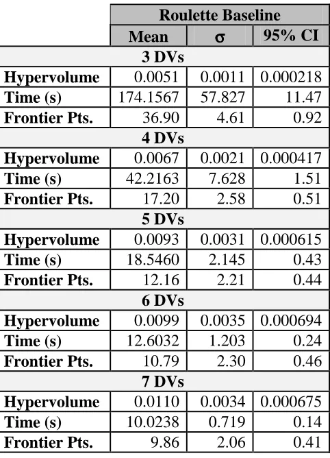
Table 3.1 UF1, 50%, 10,000 Evaluations, SI=5 Roulette Baseline Mean σσσσ 95% CI

3 DVs

Hypervolume 0.0051 0.0011 0.000218 Time (s) 174.1567 57.827 11.47

Frontier Pts. 36.90 4.61 0.92

4 DVs

Hypervolume 0.0067 0.0021 0.000417

Time (s) 42.2163 7.628 1.51

Frontier Pts. 17.20 2.58 0.51

5 DVs

Hypervolume 0.0093 0.0031 0.000615

Time (s) 18.5460 2.145 0.43

Frontier Pts. 12.16 2.21 0.44

6 DVs

Hypervolume 0.0099 0.0035 0.000694

Time (s) 12.6032 1.203 0.24

Frontier Pts. 10.79 2.30 0.46

7 DVs

Hypervolume 0.0110 0.0034 0.000675

Time (s) 10.0238 0.719 0.14

Frontier Pts. 9.86 2.06 0.41

3.3.5 Run the MOGA with Updated Selection Operator

(44)

Table 3.2. UF1, 50%, 10,000 Evaluations, SI=5 Roulette Baseline Goal Switching Mean σσσσ 95% 95% 95% 95% CI Mean σσσσ 95% 95% CI 95% 95%

3 DVs

Hyprvol. 0.0051 0.0011 0.000218 0.0055 0.0015 0.000298 Time (s) 174.1567 57.827 11.47 108.642 36.102 7.16

Fr. Pts. 36.90 4.61 0.92 34.43 4.06 0.81

4 DVs

Hypervol. 0.0067 0.0021 0.000417 0.0067 0.0023 0.000456 Time (s) 42.2163 7.628 1.51 34.1057 4.306 0.85

Fr. Pts. 17.20 2.58 0.51 18.71 2.61 0.52

5 DVs

Hypervol. 0.0093 0.0031 0.000615 0.0085 0.0028 0.000556 Time (s) 18.546 2.145 0.43 18.7182 1.717 0.34

Fr. Pts. 12.16 2.21 0.44 13.81 2.36 0.47

6 DVs

Hypervol. 0.0099 0.0035 0.000694 0.0093 0.0033 0.000655 Time (s) 12.6032 1.203 0.24 13.8523 1.099 0.22

Fr. Pts. 10.79 2.30 0.46 13.27 2.51 0.50

7 DVs

Hypervol. 0.011 0.0034 0.000675 0.0107 0.0044 0.000873 Time (s) 10.0238 0.719 0.14 11.341 1.034 0.21

Fr. Pts. 9.86 2.06 0.41 12.55 3.29 0.65

3.3.6 Compare Results

(45)

Figure 3.5. Convergence of Goal Switching and Roulette on UF1 for 3 DVs, 50%

(46)

(47)

Table 3.3. UF1, 4 DVs, 10,000 Evaluations, SI=5 Roulette Baseline Goal Switching Mean σσσσ 95% CI Mean σσσσ 95% CI

25% Selection

Hyprvol. 0.0069 0.0020 4.0e-4 0.0064 0.0022 4.4e-4 Time (s) 42.734 7.713 1.53 65.024 12.283 2.44 Fr. Pts. 16.88 2.57 0.51 21.174 3.31 0.66

50% Selection

Hyprvol. 0.0067 0.0021 4.2e-4 0.0067 0.0023 4.6e-4 Time (s) 42.216 7.628 1.51 34.106 4.306 0.85

Fr. Pts. 17.2 2.58 0.51 18.71 2.61 0.52

75% Selection

Hyprvol. 0.0069 0.0020 4.0e-4 0.0071 0.0026 5.2e-4 Time (s) 41.374 7.214 1.43 35.830 5.767 1.14 Fr. Pts. 16.94 2.62 0.52 16.95 2.71 0.54

(48)

(49)

3.4 Chapter Summary

(50)

4. GOAL SWITCHING PARAMETER ANALYSIS

4.1 Introduction

While the previous chapter defined the goal switching method and demonstrated the possible advantages, a more detailed analysis is needed to understand the effects each parameter has on algorithm performance. To reduce the computational overhead associated with the parameter study, a testing plan using design of experiments was developed. If four levels are selected for the three parameters of goal switching, 64 runs would have been needed to analyze the different possibilities. However, given the design of experiments layout shown in Table 4.1 based on a L’16 (45) orthogonal array setup, only 16 runs are needed. The

table should be read vertically for each case, with the first case having a switching mode input of 1, a cut percentage input of 1, and a switching mode input of 1. Similarly, case 10 will have inputs of 3, 2, and 4 for switching mode, cut percentage, and switching mode respectively. Tables in each subsection will describe exactly what input corresponds to each number 1-4, as this portrayal is a generic representation of the four levels chosen.

Table 4.1. Goal Switching Design of Experiments Layout

Case

1 2 3 4 5 6 7 8 9 10 11 12 13 14 15 16

Switching 1 1 1 1 2 2 2 2 3 3 3 3 4 4 4 4

Cut % 1 2 3 4 1 2 3 4 1 2 3 4 1 2 3 4

(51)

The remainder of the experimental procedure, defined in Section 3.3, is run exactly the same. For the two case study problems presented in this chapter, both roulette and tournament selection modes are used. Further analysis and conclusions related to the success of goal switching on roulette and tournament selection will be presented following the data from the case studies. The six steps are listed again below as a reminder, as they will be the template for each of the subsections in this chapter.

1) Define the problem

2) Define the assessment metrics

3) Define parameters for selection operator with goal switching 4) Run the MOGA with default selection operator

5) Run the MOGA with updated selection operator 6) Compare results

4.1.1 Design of Experiments Analysis

When the data is collected from the design of experiments runs in Table 4.1 it has to be analyzed to extract the influence that each variable had on the solution quality metrics. Further, it must be determined if the initial population used has a statistically significant effect on the results. In this setup, each case has ten unique populations, with each population being run ten times.

(52)

Table 4.1. Since there are two things that may have an effect on the outcome – initial population and the particular parameter case – analyzing the data required a two-stage nested design procedure [65]. Table 4.2 provides the formulation of the analysis of variance calculation for this type of problem setup. The first column shows the sum of the squares, the second shows the number of degrees of freedom, the third shows the mean square values, the fourth shows the F0 values, and the last shows the P values.

Table 4.2. Analysis of Variance Data Layout

Hypervolume SS DOF MS F0 P

Cases SSA DOFA MSA F0,A PA

Populations SSB(A) DOFB(A) MSB(A) F0,B(A) PB(A)

Error SSE DOFE MSE

Total SST DOFT

The equations used to fill Table 4.2 are listed below, as are the variables and their associated meanings.

a = cases (1-16, baseline, 17 total) b = populations (1-10, 10 total)

n = runs (1-10, 10 total) y... = Total (sum of case totals)

(53)

yijk = Run value

SS

_A

=

1

bn

∑

y

i.. 2

_-

y…2

abn a

i=1

(4.1)

SS

_B(A)

=

1

n

∑ ∑

y

.

2

+

-bn a

i=1

∑

.-=1,_-..2 (4.2)

SS

_E

=

∑ ∑

+

∑

/

,

-n a

i=1

∑ ∑

.-=1 0=1,_{- .}2 (4.3)

SS

T

=

∑ ∑

ai=1 +

∑

/

,

-

_2+/1…%

(4.4)

34 5 = . − 1

(4.5)

34 6(5) = .(0 − 1)

(4.6)

34 7 = .0( − 1)

(4.7)

34 8 = .0 − 1

(4.8)

9:5 = ::5⁄34 5

(4.9)

9:6(5)= ::6(5)⁄34 6(5)

(4.10)

9:7 = ::7⁄34 7 (4.11)

F0 is for fixed A and B [65]

<,5 = 9:5/9:7

(4.12)

<,6(5) = 9:6(5)/9:7

(4.13)

P-Values were determined using the fcdf command in Matlab [64], which is a cumulative distribution function. The inputs are F0,A, DOFA, and DOFE for P-0A and F0,B(A), DOFB(A),

(54)

To be considered a statistically significant result the P-Value of a row should be low (less than 5%). For example, if PA is less than 0.05, there is a 95% likelihood that a change in the

measured outcome is impacted by the case being run. If the value of PB(A) is low, then the

initial population used has an effect. The higher the percentage in the P column, the less likely the corresponding variable had an effect on the final outcome.

4.1.2 Main Effects and Linear Model Fit

(55)

Figure 4.1. Example Main Effects Plot

As in the previous section, there is a relationship between the index used to represent the x-axis in the main effects plot and the true value for each parameter. For reference, an example of this mapping relationship is shown in Table 4.3.

Table 4.3. Example Mapping Relationship between Index Number and Parameter Setting

1 2 3 4

Switching (gen.) 3 5 10 20

Cut % 25 50 75 100

(56)

The results from the linear model fit, whose form is shown in Equation 4.14, will be shown in table form. In equation 4.14, β represents the parameter being estimated, X represents the value of that parameter, and ϵ represents the error.

> = ?<+ ? @ + ? @ + ⋯ + ?/@/+ B (4.14)

In such tables, the first setting for each parameter is omitted. This omission is done because the model is fit using a dummy-encoding scheme. Under this scheme, it is assumed that the value of the first setting for each parameter is 0, establishing a baseline by which to measure the impact of changing the value of the parameter. Further, the intercept value reports the estimate of the performance metric when these baseline settings are used.

As shown in Table 4.4, every parameter besides the baseline is reported by including both a P-Value and an estimate of the coefficient (β). Here, the P-Value is significant if the value

is less than 5%. The estimate of the coefficient reports if that particular parameter value has a positive or negative effect on the performance metric being measured. The strength of this effect is represented by the magnitude of that number.

(57)

Table 4.4. Example Linear Model Fit Data Layout

Hypervolume Estimate Se Tstat Pvalue

Intercept 0.449139 0.003734 120.2785 0

5 Switch -0.00452 0.003207 -1.41E+00 0.158764 10 Switch -0.01701 0.003734 -4.55445 5.65E-06 20 Switch -0.02293 0.003312 -6.92121 6.47E-12 50% 0.005247 0.003448 1.521793 0.12826 75% 0.005972 0.003448 1.73231 0.083412 100% 0.005838 0.003448 1.693214 9.06E-02 C1 -0.00625 0.003312 -1.88536 0.059563 C2 -0.0132 0.003448 -3.8291 0.000134 C3 -0.01693 0.003312 -5.11097 3.59E-07

Having defined the mathematical foundation of the analysis needed for this chapter, the following sections explore the effect of goal switching in two case study problems.

4.2 CASE STUDY 1 – MP3 Player Product Line Design Problem

This section explores the design of an MP3 player product line where the objectives of the problem are two maximize a surrogate of price and market share of preference. Each sub-section corresponds to the six step experimental procedure introduced in Chapter 3.

4.2.1 Define the Problem

(58)

measure of profit. Analyzing these two objectives requires a mathematical representation of customer preference for the different product components that the company can choose from and the price of each product in the line. To get this information, customer reference data was obtained using a choice-based conjoint survey using Sawtooth Software SSI Web [66]. Table 4.5 shows the breakdown of the seven product attributes and the price levels used in the survey.

Table 4.5. MP3 Player Attributes and Price Levels

Levels Photo/ Video/ Camera Web/ App/ Ped

Input Screen

Size Storage

Background Color

Background

Overlay Price

1 None None Dial 1.5 in

diag 2 GB Black

No pattern / graphic overlay

$49

2 Photo only Web

only

Touch-pad

2.5 in

diag 16 GB White

Custom pattern overlay

$99

3 Video only App only Touch-screen

3.5 in

diag 32 GB Silver

Custom graphic overlay $199 4 Photo and Video Only

Ped only Buttons 4.5 in

diag 64 GB Red

Custom pattern and graphic overlay $299 5 Photo and lo-res camera Web and App only 5.5 in

diag 160 GB Orange $399

6 Photo and hi-res camera App and ped only 6.5 in

diag 240 GB Green $499

7 Photo, video and lo-res camera Web and

Ped only 500 GB Blue $599

8

Photo,vide o and hi-res camera

Web, app, and

ped

(59)

To get mathematical representations of customer preference for each feature and price level, a hierarchical Bayes (HB) mixed logit model was fit using Sawtooth Software CBC/HB [67] to estimate the observed part-worths for each respondent. The data used to fit the model came from 205 choice-based conjoint surveys containing twelve choice tasks each. This model was fit using the default settings and the part-worths for the price levels were constrained to be monotonically decreasing (i.e. the part-worth for $49 is greater than the part-worth for $99). For each of the 205 respondents, fifty-five total part-worths are calculated: forty-six for the features, eight for the price levels, and one for the outside good. The outside good is the share of the combined shares of the inside goods subtracted from the total potential market size.

Estimating market share of preference [68] is done by predicting the probability (C) that a respondent will select a certain product over the rest of the field. In Equation 4.15, the

probability of selecting the -DE product is predicted by dividing the exponential of the observed utility (F) of the -DE product by the sum of the exponentials of all products under consideration (including the outside good). A respondent’s share of preference for a product line is merely the summation of all the individual product preference shares. This value can then be aggregated across all respondents in the survey to get a market share of preference of the product line.

C =_{∑ G}_/GHI _H_J (4.15)

(60)

used only includes the feature cost of the product being sold. Contribution margin is the difference between a product’s selling price (K) and its cost (L); it does not account for investments, other fixed costs, or the time value of money. Equation 4.16 shows the

formulation of the per capita contribution margin for the -DE product in the product line. To get the PCCM for a product line, simply sum the PCCM for each product.

KLL9 = (K − L ) ∗ C (4.16)

(61)

Table 4.6. MP3 Player Cost Per Feature

Levels Photo/

Video/ Camera

Web/ App/ Ped

Input Screen

Size Storage

Background Color

Background Overlay

1 $0.00 $0.00 $0.00 $0.00 $0.00 $0.00 $0.00

2 $2.50 $10.00 $2.50 $12.50 $22.50 $5.00 $2.50

3 $5.00 $10.00 $20.00 $22.50 $60.00 $5.00 $5.00

4 $7.50 $5.00 $10.00 $30.00 $100.00 $5.00 $7.50

5 $8.50 $20.00 $35.00 $125.00 $5.00

6 $15.00 $15.00 $40.00 $150.00 $5.00

7 $16.00 $15.00 $175.00 $5.00

8 $21.00 $25.00 $200.00 $10.00

As the firm would ideally like to maximize both of these objectives, they are reformulated into minimizations by multiplying by negative one. Further, it was decided that the company would design five products for the line. This decision led to a problem formulation with 81 design variables: 46 price markup variables (continuous variables between 0 and 1) and 35 product configuration variables (7 per product represented as integer variables).

4.2.2 Define the Assessment Metrics

(62)

4.2.3 Define Parameters for Selection Operator with Goal Switching

To accommodate the design of experiments structure shown in Table 4.1, 4 different values of each of the three parameters were chosen. Each value can be seen in Table 4.7, and these values correspond to the numbers 1-4 on the main effects plots for this problem. The first variable is switching index as a function of generations (Switching), the second is selection percentage (Cut %), and the last is switching mode (Mode).

Table 4.7. Design of Experiments MP3 Reference

1 2 3 4

Switching (gen.) 3 5 10 20

Cut % 25 50 75 100

Mode f1,f2 f1,f2,both f1,both,f2 f1,both,f2,both

Switching index was bounded between 3 generations and 20 generations so the effect of quickly switching or slowly switching could be observed. The generation limit was set to 100, so a switching index of 20 cycles through each of the objectives once for the (f1, both, f2, both) case and leaves a few generations at the beginning for burn-in. Having a lower

(63)

4.2.4 Run the MOGA with Default Selection Operator

For each experiment in Table 4.1, 10 replications were run for 10 unique starting populations. Objective 1 is the normalized market share of preference (originally from 0% to 100%) and objective 2 represents the surrogate measure of profit (PCCM). The settings for the MOGA used in this study were:

• Population size: 10*number of design variables

• Encoding: real-value and integer • Crossover type: scattered crossover

• Crossover rate: 50%

• Mutation: linearly decreasing rate starting at 5% and ending at 0% • Convergence: 80,000 function evaluations

(64)

Table 4.8. Baseline Results, MP3 Problem

Hyp. σ CI Frnt.Pts. σ CI Crd.Dst. σ CI

Roulette 0.4525 0.015 2.98E-03 113.86 10.9034 2.16 0.0783 0.0083 1.65E-03

Tourn. 0.4099 0.0147 2.92E-03 233.76 29.9479 5.94 0.05 0.0077 1.53E-03

The hypervolume and crowding distance should be minimized for optimum results and the frontier points should be maximized for the same reason. Here it is easy to see that the tournament selection method is more effective at finding frontier points as well as minimizing hypervolume and crowding distance.

4.2.5 Run the MOGA with Updated Selection Operator

(65)

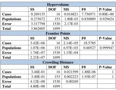
Table 4.9. MP3 Roulette Selection Analysis of Variance Results Hypervolume

SS DOF MS F0 P-Value

Cases 0.269135 16 0.016821 7.756971 0.00E+00

Populations 0.275672 153 1.80E-03 0.830889 0.929624

Error 3.317798 1530 2.17E-03

Total 3.862605 1699

Frontier Points

Cases 3.42E+06 16 2.14E+05 18.5785 0

Populations 1.07E+06 153 6.97E+03 0.60527 0.999947

Error 1.76E+07 1530 1.15E+04

Total 2.21E+07 1699

Crowding Distance

Cases 3.46E-01 16 0.021599 1.88E-06 1

Populations 3.40E-01 153 0.002223 1.93E-07 1

Error 4.12E+00 1530 0.00269

Total 4.80E+00 1699

In Table 4.9 it can be seen that the change in hypervolume and frontier points is statistically significant when the case is changed, but not when the population is changed. This is desired as the outcome of the results will not be influenced by the starting points but rather the process of selection. However, for crowding distance, neither the case used or the starting population have a statistically significant impact on the results.

(66)

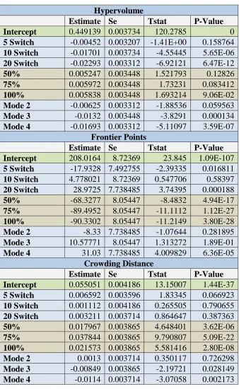
Table 4.10. MP3 Roulette Selection Linear Fit Results Hypervolume

Estimate Se Tstat P-Value

Intercept 0.449139 0.003734 120.2785 0

5 Switch -0.00452 0.003207 -1.41E+00 0.158764 10 Switch -0.01701 0.003734 -4.55445 5.65E-06 20 Switch -0.02293 0.003312 -6.92121 6.47E-12 50% 0.005247 0.003448 1.521793 0.12826 75% 0.005972 0.003448 1.73231 0.083412

100% 0.005838 0.003448 1.693214 9.06E-02

Mode 2 -0.00625 0.003312 -1.88536 0.059563

Mode 3 -0.0132 0.003448 -3.8291 0.000134

Mode 4 -0.01693 0.003312 -5.11097 3.59E-07 Frontier Points

Intercept 208.0164 8.72369 23.845 1.09E-107 5 Switch -17.9328 7.492755 -2.39335 0.016811 10 Switch 4.778021 8.72369 0.547706 0.58397 20 Switch 28.9725 7.738485 3.74395 0.000188 50% -68.3277 8.05447 -8.4832 4.94E-17 75% -89.4952 8.05447 -11.1112 1.12E-27

100% -90.3302 8.05447 -11.2149 3.80E-28

Mode 2 -8.33 7.738485 -1.07644 0.281895

Mode 3 10.57771 8.05447 1.313272 1.89E-01

Mode 4 31.03 7.738485 4.009829 6.36E-05

Intercept 0.055051 0.004186 13.15007 1.44E-37 5 Switch 0.006592 0.003596 1.83345 0.066923 10 Switch 0.001112 0.004186 0.265505 0.790655 20 Switch 0.003211 0.003714 0.864647 0.387363 50% 0.017967 0.003865 4.648401 3.62E-06 75% 0.037844 0.003865 9.790807 5.09E-22

100% 0.021573 0.003865 5.581416 2.80E-08

Mode 2 0.0013 0.003714 0.350117 0.726298

Mode 3 -0.00849 0.003865 -2.19721 0.028149

(67)

Figure 4.2. MP3 Hypervolume Main Effects Plot, Roulette Selection

(68)

Figure 4.4. MP3 Frontier Points Main Effects Plot, Roulette Selection

(69)

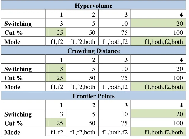
with the same settings. Table 4.11 shows a summary of results for the goal switching with roulette selection operator. Comparing the winners in Table 4.11 to Table 4.10, the switching index and switching mode both are significant for the hypervolume since they have a Pvalue below 5% compared to the baseline. For crowding distance, switching mode 4 is under 5% for the Pvalue so is significant with respect to the baseline goal switching case. Again, 25% cut percentage is on the baseline. Finally, switching index and switching mode are significant with respect to the baseline for the number of frontier points, but cut percentage is on the baseline goal switching case.

Table 4.11. MP3 Main Effects Plot Summarized Results, Roulette Selection

Hypervolume

1 2 3 4

Switching 3 5 10 20

Cut % 25 50 75 100

1 2 3 4

Switching 3 5 10 20

Cut % 25 50 75 100

Frontier Points

1 2 3 4

Switching 3 5 10 20

Cut % 25 50 75 100

(70)

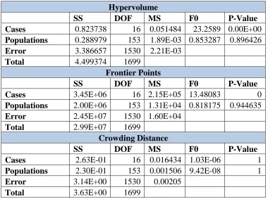
significantly changed by the cases and not the populations. Also, crowding distance is not changed in a statistically significant way by altering the cases or the populations.

Table 4.12. MP3 Tournament Selection Analysis of Variance Results Hypervolume

Cases 0.823738 16 0.051484 23.2589 0.00E+00

Populations 0.288979 153 1.89E-03 0.853287 0.896426

Error 3.386657 1530 2.21E-03

Total 4.499374 1699

Frontier Points

Cases 3.45E+06 16 2.15E+05 13.48083 0

Populations 2.00E+06 153 1.31E+04 0.818175 0.944635

Error 2.45E+07 1530 1.60E+04

Total 2.99E+07 1699

Cases 2.63E-01 16 0.016434 1.03E-06 1

Populations 2.30E-01 153 0.001506 9.42E-08 1

Error 3.14E+00 1530 0.00205

(71)

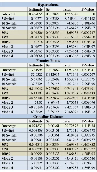
Table 4.13. MP3 Tournament Selection Linear Fit Results Hypervolume

Intercept 0.469055 0.003829 122.5141 0

5 Switch -0.00271 0.003288 -8.24E-01 0.410198 10 Switch -0.01792 0.003829 -4.6806 3.10E-06 20 Switch -0.02875 0.003396 -8.46472 5.75E-17 50% -0.01306 0.003535 -3.69538 0.000227 75% -0.02179 0.003535 -6.16451 8.95E-10

100% -0.0316 0.003535 -8.93865 1.07E-18

Mode 2 -0.01675 0.003396 -4.93081 9.05E-07 Mode 3 -0.02562 0.003535 -7.24664 6.64E-13 Mode 4 -0.03068 0.003396 -9.03362 4.69E-19

Frontier Points

Intercept 139.4995 10.02682 13.91263 1.31E-41 5 Switch -32.0322 8.612015 -3.71948 0.000207 10 Switch 15.57365 10.02682 1.553198 0.120575 20 Switch 37.8125 8.89445 4.251246 2.25E-05 50% 6.866042 9.257637 0.741662 0.458401 75% 16.14104 9.257637 1.743538 0.081433 100% 44.83104 9.257637 4.842601 1.41E-06

Mode 2 24.02 8.89445 2.70056 0.006996

Mode 3 68.70146 9.257637 7.421057 1.88E-13 Mode 4 63.7625 8.89445 7.168796 1.15E-12

(72)

(73)

Figure 4.7. MP3 Frontier Points Main Effects Plot, Tournament Selection

From Figures 4.5 and 4.7 the optimum variable inputs for hypervolume and number of frontier points can be seen to be the same as the roulette operator: a switching index of 20, a cut percentage of 100%, and a switching mode of (f1, both, f2, both). Crowding distance is almost the same, with switching mode being almost even between (f1, both, f2, both) and (f1, both, f2). More than likely they could all be optimized together, especially since changing the

(74)

percentage is on the baseline. The crowding distance is the only parameter to be significant with respect to the baseline for the crowding distance metric.

Table 4.14. Main Effects Plot Summary Tournament MP3

Hypervolume

1 2 3 4

Switching 3 5 10 20

Cut % 25 50 75 100

1 2 3 4

Switching 3 5 10 20

Cut % 25 50 75 100

Frontier Points

1 2 3 4

Switching 3 5 10 20

Cut % 25 50 75 100

4.2.6 Compare Results

(75)

has a worse score than the baseline in cases 3, 7, 11, 15, and 16, but still achieves a higher score more than 66% of the time.

Data for the tournament method is not nearly as strong, with the hypervolume and frontier points only having higher than baseline results 4 of 16 times, and crowding distance only scoring higher than the baseline 3 of 16 times. It is unclear why goal switching does not work as well on tournament for this specific problem.

Table 4.15. MP3 Roulette Mean Analysis

Hyp σ CI Frnt.Pts σ CI Crd.Dst σ CI

1 0.4567 0.0257 5.10E-03 209.40 45.0575 8.94 0.0557 0.0103 2.04E-03

2 0.4417 0.0136 2.70E-03 144.96 21.3253 4.23 0.0735 0.018 3.57E-03 3 0.4385 0.0105 2.08E-03 133.05 15.9428 3.16 0.08 0.0205 4.07E-03 4 0.4403 0.0091 1.81E-03 129.78 10.7705 2.14 0.0698 0.0075 1.49E-03 5 0.4390 0.0157 3.11E-03 163.54 37.5169 7.44 0.0638 0.0095 1.88E-03 6 0.4463 0.0083 1.65E-03 136.37 11.0012 2.18 0.0764 0.0168 3.33E-03 7 0.4370 0.0159 3.15E-03 132.44 17.273 3.43 0.0857 0.0188 3.73E-03 8 0.4333 0.0078 1.55E-03 135.88 18.2172 3.61 0.0744 0.0135 2.68E-03 9 0.4351 0.0152 3.02E-03 177.89 26.1544 5.19 0.0581 0.0077 1.53E-03 10 0.4267 0.0199 3.95E-03 154.01 22.0058 4.37 0.067 0.0134 2.66E-03 11 0.4321 0.0079 1.57E-03 129.35 23.2894 4.62 0.0953 0.016 3.17E-03 12 0.4314 0.0108 2.14E-03 129.57 15.1432 3.00 0.0735 0.0145 2.88E-03 13 0.3974 0.0109 2.16E-03 307.62 58.5387 11.61 0.0404 0.0066 1.31E-03 14 0.4220 0.0066 1.31E-03 172.51 25.565 5.07 0.0675 0.0124 2.46E-03 15 0.4320 0.0094 1.86E-03 128.34 21.843 4.33 0.1029 0.0266 5.28E-03 16 0.4341 0.0104 2.06E-03 124.61 14.667 2.91 0.0811 0.0169 3.35E-03