Volume 20, Number 5 (September 1967)

(1)

(2)

(3)

(4)

Jmmd of RANGE MANAGEMENT vozgzs$%,e7

5

Ediforial. The Trail Boss _._._____.______.__ . . .._. _ _... ________._______.__ _.__ . . . ..Harold F. Heady Rangelands-Challenge to the Pockefbook... _______ M. L. Upchurch Geographic Disfribufion and Factors Affecfing fhe Disfribufion of Salf

Deserf Shrubs in fhe Unifed Sfafes..._._._ ____ ________._ _____ ____._______ F. A. Branson, R. F. Miller, and I. S. McQueen Grazing Distribufion Patterns of Hereford and Santa Gerfrudis Catfle on a

Soufhern New Mexico Range ______________________.____________I____.__ ._.. _________.._._____ _._.__ _ .__.___. Carlton H. Herbel, Fred N. Ares, and Arnold B. Nelson Influence of Temperafure on the Germinafion of

Some Range Grasses _______ ___ _____ ______._ ____ ____._______.___ .__. . . ..O. D. Knipe Potenfial for Increases in Grazing Fees..._... ____ . . . ..Jack F. Hooper Whaf is Range Managemenf?..._.___.._.._.._..~~.~~L. A. Stoddart Response of Forage Grasses fo Rhodesgrass Scale...Michael F. Schuster Comparison of Tropical Forages of Known Composifion with Samples of

These Forages Collecfed by Esophageal Fisfulafed Animals... . .._____..___.. B. Marshall, D. T. Torell, and R. M. Bredon Variation of Esophageal Fisfula Samples Between Animals and Days on Tropical Grasslands_ _____________ . . ..D. T. Tore& R. M. Bredon and B. Marshall Measuremenf of Selecfive Grazing of Tropical Pastures Using Esophageal Fistulafed Sfeers ____ _ ___________ _ ____ . ..R. M. Bredon, D. T. Tore11 and B. Marshall Germinafion of Foresf Range Species from Soufhern

Brifish Columbia_ ___. ___ ____ _____ ________ _ _____ __ _..____.___ _ ___________ ___________ __.__ ..Alastair McLean The Sampling Unit and Ifs Effect on Salfbush Yield Esfimafes....J. ROSS Wight Range Managemenf in fhe Libraries of North America...F. P. Cronemiller Range Managemenf Theses 1966-Compiled and Edifed by Ervin M. Schmufz Technical Nofes:

Relafive Germinafion of Spoffed and Nonspoffed

Bifferbrush Seed.. _.________ _ _______ _ ___________.____ ______ _________ ____ ___. Robert B. Ferguson Weighing Forage Samples on Windy Ranges...Richard S. Bjerregaard Effecf of Delays in Inoculum Collecfion on Ariificial Rumen

Digesfibilifies... ____ ____________ __.___ _ .__.___. ____ ____ ________ __.__._ _ _._. _ __.. Henry A. Pearson Managemenf Nofes:

Wafer Requiremenfs for Improved Livesfock Performance ’ on ~angeland...~..~.__~ .._.__._.____ _ ..___._ . ..Samuel F. Greenfield Book Reviews:

Sysiems Analysis in Ecology (George M. Van Dyne)... .._. _ . . . _ .__...-. _ . . . . ..-.. New Publicafions

News and Nofes... ____ ______ _____ ______________________________~~~_._~~..__.~..~_~~ ____.____..._...._.-..-.-. -.._.---.._._

Wifh fhe Sections.. ____ _____.__.________________________ _____ ___._____ _..._ ______ ____.______________._..______.___.-..--..--.--.- Society Business... ____ ___________.__.______________________..______._...___ _.._ ________._ .___ _ _...__..._._.__._---.- -.-.---

336 339 341 283 284

287

296

298 300 304 307

310

314

317

321 323 326 329

330 331

332

333

335

Cover

Photo-_

Wafer for Livestock

Performance

(5)

Editorial

The Trail Boss

HAROLD F. HEADY

Professor of Forestry (Range Man-

agement), University of California, Berkeley.

Since “The Trail Boss” became the Society’s trade mark, I have wondered at the image it por- trays and have heard various opinions expressed. The one I prefer is the Boss’s dedication to a job and his determination to reach his goal no matter the set backs from storm, fire, and Indians. All will agree that the image of putting out all that he has to reach his objective in the face of adversity is a fitting motto for the Society and for us as individuals.

Also the emblem may suggest to some that the range management objective has concern with livestock. If the concern is only with livestock, I believe that the image is much too narrow. It is this area of range management objectives to which the follow- ing remarks are addressed.

Range managers, because of the breadth of their training and their job responsibilities, are land managers. Their concern is with all the resources of the land. They are practicing ecologists in a broad sense, as they are concerned with the whole of the landscape, the production of goods and services from the landscape, and man’s impact on the landscape. The range manager is vitally concerned with the impact of consumer organisms on the landscape, including domestic animals, wild animals, and man himself. Recently increased importance of wild animals and of recreational man in the rangeland setting needs further recog- nition. This leads me to suggest that the range manager should exercise initiative and leadership in rangeland management where the objective is more than livestock production. He has the fundamental knowledge and experience to accomplish efficient land use of several types.

The range man’s animal management problems and solutions are centered on 5 principles. They are correct stocking rate, season of use? frequency of use, kind of animal, and distribution of animals. These are so widely known and applied in livestock management that it may be trite to repeat them. I do so for the purpose of emphasizing that much in successful game-range management depends on the same five principles. Range management is still range management whether the animals used are domestic or wild. It seems to me that the range manager’s knowledge and experience in using these principles of man- aging the influence of animals on their food and cover resources is as vital to game management as it has been to successful range livestock management.

The relatively new and rapidly expanding field of wildland recreation can use these same principles. Man as a camper, hiker, and hunter in wildland situations exerts pressures on wild lands in terms of his numbers, season of use, frequency of use, kind of use, and his distribution. Many problems of recreational use are problems within these five areas. Their solutions lie in the application of concepts with which the range man is already familiar and experienced. It is a short step from rotation of grazing to rotation of camp grounds and the rotation of trampling by human feet. The increasingly critical problem of recreational horse grazing is a range problem which should be solved by range people.

Range managers are concerned with the manipulation of vegetation as much as they are with animals. Very large bodies of information on seeding, control of noxious plants, fertilization, and soil conservation prove this point conclusively. Game management and recreational management are also concerned with manipulation of natural vegetation. Range managers can and do con-

283

tribute to these fields but I believe the changing demands on our wild lands gives us a largely untaken opportunity to be more effective as land managers. Man- agement of vegetation for game and recreational purposes is a new challenge demanding vision- ary thinking which range people can provide.

The purpose of the Society, as stated in every Journal issue, can be interpreted to include the uses of wildland for game and recreation but it takes some word-twisting to do so. “The science and art of grazing land management” could include recreational areas but I believe our profession is saying too frequent- ly that these are no longer “grazing areas” when actually they are areas “grazed” by man. “. . . sustained use of forage, soil and water resources” again confines the application of our subject matter facility too closely to the livestock industry by the choice of the word “forage.” “. . . sustained use of vegetation, soil and water resources” would be more suitable. The Society’s objectives need revising.

These comments do no injus- tice to the fact that range management has a principle orienta- tion toward livestock, but growing “conflicts” over the use of rangeland for domestic animals, game animals, and recreational purposes will not be solved in the best interests of all land users until the range manager applies his special facility in solving those problems. We need to stimulate our interest and increase our influence in all wildland management problems.

(6)

Rangelands-Challenge

fo the Pocketbook1

M. L. UPCHURCH

Administrator, Economic Research Service, U.S.D.A., Wa.shington, D.C.

Highlight

Rangeland users can expeci to share in the growing market for beef in the next 20 years. But they may face increasing competition from other types of producers. Good range management in the future will re- quire prudent investment and the ability fo benefit from business man- agement and partial ownership of resources.

Any rancher who has fed $60 hay to $80 cows and has avoided foreclosure on a piece of rangeland during tough years does not

need to be reminded of chal-

lenges to the pocketbook, Cer-

tainly, there have been challenges in the past and there will be others in the future. Since

man first domesticated animals,

the rangeland user has had to face the challenges of nature and the challenges of the economic and social environment in which he found himself. Both, at times, seemed to conspire against him;

occasionally both smiled in his

favor.

The “Pocketbook” problems of

rangeland use during the next 20 years will be closely linked with the economics of the beef cattle industry. Sheep, wildlife, watershed, recreation, and other uses of rangeland will all play their part, but the cow business predominates most range use.

In looking at past and probable future trends in the consumption of beef, it is easy to become op- timistic about the economic future of beef ,producers. Popula- tion is increasing and will continue to increase. Per capita incomes are increasing and likely- will continue to grow. Both factors increase the total demand for beef. The taste for beef, a

IPaper presented .at Annual Meeting, American Society of Range Manage- ment, Seattle, Washington, Febru- ary 13-16, 1967.

relatively expensive food, seems to grow with increasing incomes. So the outlook for growth in the beef business seems probable in the long run.

These probable trends for the next 20 years suggest optimism about the future of the rangeland owner and user. Grain is a rela-

tively cheap resource in the

United States and likely will remain so despite the growing ex- port demand and the need for grain for direct human consumption. With relatively cheap grain, and with our growing taste for grain-fed beef, the demand for feeder animals through which grain is marketed would appear

to be increasingly strong. At

times in the past we have seen feeder cattle bring more on the market than finished cattle; the

livestock feeder operated on a

negative margin. Such price relationships may occur more fre-

quently in the future. Feeder

animals are a major product of rangeland. In such a setting, one

could conclude that the range

user’s role would be simply a judicious expansion of inputs on the range. Thus, the rancher could feel confident of an increasing estate and a comfortable re- tirement in 20 years.

But this does not mean that all beef producers are going to make money all the time ,during the next 20 years. Even with a gen-

eral strengthening demand for

beef, producers of feeder stock and producers of slaughter animals will continue to face chal-

lenges to their pocketbooks as

costs of production and price relationships vary over time.

Range users will have opportunity to participate in expanding production of feeder cattle. But they will not necessarily be

in a dominant position. The

range is not the only place where feeder cattle can be raised. Beef

cattle production has expanded

in almost all regions of the

United States, including areas

predominated by crop farming,

dairying, and specialty crop production. Recently we have seen a great expansion in beef cow numbers in the South and Southeast. Throughout the United States we have a great potential for beef cattle raising using many different types of feed. So the beef producer who uses rangeland

will compete increasingly with

producers who use other types of feed resources.

Despite this competition, we

will continue to have (at least for the next 20 years) vast acreages of land used for the production of grazing animals. About half the total land area of the continental United States is now used for this purpose. Most of our present acreages of rangelands are used for livestock grazing now because they are either not suitable for or are not needed for other purposes. Simply, un- der present economic and tech-

nological conditions we have

about a billion acres of land that are managed most profitably by

permitting grazing animals to

harvest the forage produced. Only in this way can the forage from such land be economically

collected, concentrated, trans-

ported, and converted into a

product suitable for human use. But this condition may not per- sist universally and indefinitely. Our rangelands of today are gen-

erally residual lands; that is,

they are lands that no one else wants or needs for more intensive uses in our present economic

environment. By selection over

the years we have reserved for other uses the lands most re- sponsive to intensive inputs, and, on the other hand, we have left to range use the lands least re- sponsive to intensification.

This process of selection is a perfectly normal result of the operations of an economic and social system where men have had the freedom to choose how to use the resources at their disposal. This process of selection, however, raises some interesting

(7)

questions about the future nomic use of rangeland.

eco-

As our market for beef con- tinues to grow in the long run,

what is the potential for the

range stock producer to intensify

production in competition with

producers using other types of

resources? During the past 30

years we have learned much

about how to make rangelands more productive. Better grasses,

better techniques for livestock

management, w at e r develop- ment, fencing, brush control, and a host of other practices have been developed and brought into common use. Much improvement has been made, and further im-

provements are possible and

likely. However, the rangeland

user must not forget that he is dealing with a resource that has relatively low capacity to absorb

inputs profitably. Thus, the

rangeland user m u s t calculate carefully the response he can ex-

pect from added investments in

range improvements and the

risks of such investments, and he should compare expected returns with those he might get from al-

ternative investments. Specifi-

cally, if a rancher has $5,000 to invest, should he reseed a section of range, or should he improve the irrigation system for his hay meadows? The answer, of course,

depends on circumstances in

each individual case. Generally, we find that added investments pay off best when applied to the most productive land. Similarly, an investment in beef-producing capacity on good farmland may yield more beef per dollar input

than a like investment on low

yielding range.

This does not mean that in-

vestments for range improve-

ments will not continue to be

made. They will be. It does mean that ranchers, or the public, who make such investments must be continually prudent to avoid mis- use of resources. As land becomes more costly, the chance for er- rors that put the range livestock

RANGELANDS-POCKETkOOK 285

business in the red instead of the black becomes greater.

The technology of livestock

production, whether on the farm or the ranch, is becoming increasingly sophisticated. Breeding and

management of both sheep and

cattle have been steadily im-

proved. Drugs to increase inci- dence of twins, to regulate breeding cycles, and to speed growth rates are now known and could

come into common use in the

years ahead. To make the most

of these advanced techniques

will require increasing attention to livestock nutrition. Thus, we may see a time when we cannot afford to use low-capacity range

for high-capacity livestock. In

this case, we may very well find it more profitable to concentrate livestock production on our better land and on harvested feeds, while we leave the poorer range-

land to game, recreation, and

watershed purposes.

In common with trends

throughout agriculture, we can

expect ranches of the future to be larger and fewer in number. The usual reason given for increasing the size of a ranch is to reduce unit costs of production. While it is true that some ranches are inef- ficiently small, the chief reason for the trend toward larger units is to provide the rancher with

more total income whether or

not unit costs are decreased. Most ranchers, like nearly every-

one else, want more income. If

they can increase their individual incomes by running a 500- head spread, rather than 300 head, they will do so. Modern equipment makes it possible for a man to handle more land and more animals than he did 20 years ago. With this possibility, size of ranches will continue to increase.

Traditionally we have thought

of the range livestock producer

as a combination entrepreneur,

laborer, and investor. He wore

three hats. As an entrepreneur he decided what resources were

to be used and he made the management decisions. His role as a

self-employed laborer was obvi-

ous. He was also an investor to the extent that he had his own money in the assets of the business.

In the future, the rancher may become more the entrepreneur

and less the investor. This

change will come as a result of

economic forces and trends in

prices of ranch property. These trends have been going on for the past 75 years, and I expect they will continue for another 20. This suggests that we take a long look at the traditional roles

of the entrepreneur, the asset

owner, and the investor in the ranching business.

Let us start with the investor. An investor is one who has a money equity in a production good, whether the good be rangeland, the cattle grazing on it, or

the ranch equipment. The in-

vestor need not also be the owner of the good; he may be the mortgage holder. Investors are those who desire to obtain an interest

return on their money. An in-

vestor may also be the owner in which case his investment is represented by his equity in the land and other property. His return as an investor is the mortgage rate of interest. This is the “opportunity cost” of his invest-

ment because presumably, he

could put his money in some

other business and earn the going rate of interest.

The owners of production

goods obtain their returns in the form of contractual rents, which

are based on “economic rents.”

These, in turn, are based on, but not equivalent to, the value of

the product attributable to the

(8)

286

hand, owners may have very little of their own money “invested” in the resources they own. In this case they are interested chiefly in the ownership return - rather than the investor’s return.

Entrepreneurs obtain their returns in the form of profits which result from a production process. Profits represent the difference between the value of the product derived from a resource and the contractual rent or charge for that resource. An entrepreneur may or may not choose also to be an owner of resources or an investor in them depending upon how he views the prospective value of the rent. Sometimes entrepreneurs prefer to vie for the profits of entrepreneurship rather than the rents of a landlord or the interest of the investor.

Let me illustrate the above re- lationship. Suppose we have an acre of meadow worth $100; the rent is $10; the mortgage interest is $6; it produces a net value . product of $20 (including rent). In this example the entrepreneurial return is $10 ($20 value product minus $10 rent). The ownership net return is $4 ($10 rent minus $6 interest) the investor’s return is $6.

Why, you may ask, would anyone prefer the $4 net to ownership over the $6 net to investment? The reason is clear when you consider that for a 20% equity, or $20, an owner after paying $4.80 in interest on the $80 mortgage would realize a net of $5.20 as an owner, or 26% on his investment.

The entrepreneur earns and receives his managerial profit whether or not he “owns” the production resource. Ownership is not essential but it does give the entrepreneur a measure of security in a continuing business, Although it is not essential, many entrepreneurs and typically ranchers prefer to “own” their resources. But ownership,

UPCHURCH

as we have seen, is not synony- mous with investment. A rancher can participate in the advantages of ownership without being a 1003 investor. The decision on whether and how much to invest is a separate matter from ownership or from entrepreneurship.

At one time, and perhaps until recently, it generally was prudent for operating ranchers to “invest” their own earnings and savings in the ranch properties they used. Many strove to increase their equities as fast as possible. These properties were perhaps as good as any other kind of investment. Nowadays it is becoming more doubtful whether ranch properties are a good, or I should say, the best investment for the operating

rancher. The reason for this

question is not because the properties are no longer productive. They are highly productive. The reason is because they are over- priced in today’s market, over- priced, that is, for the operating

rancher based on returns from

production.

I have no completely satisfac- tory explanation for the price of ranch properties. Often current land values are not justified by current levels of economic rent. There are several other factors affecting the present price of land. For one, there are buyers who are more interested in long- term gains or value appreciation than in current return on current values. This situation is analo- gous to the “growth” stocks of the financial market in which the investor hopes for increased value of stocks more than current divi- dends. Some ranch properties are returning as little as 1 or 2% on current values. These long- term investors hope to recoup in rising land values, what they forgo in the way of current returns on investment. Most operating ranchers are not able to play that kind of game. They need their financial resources for upgrading their day-to-day op-

erations, .for improving produc- tivity and efficiency of current operations.

This being the case, the best current strategy for the operating ranchers is to let someone else, the bank or another individual, carry most of the long- term investment. One challenge of the next 20 years to the operating rancher will be to accept this new role; that is, the role of the operating entrepreneur as distinct from the role of investor.

We are thinking of an operating manager who has a minimum equity in the ranch real estate, who is satisfied to let someone else (a banker or individual) accept a relatively low rate of return on his investment, and is willing to pay that charge. In doing this, the rancher can keep his own money invested in operating capital - better bulls, good winter rations, adequate equipment, range improvements, and so on, in which the value product is greater and for which the loan rate of interest is higher than for land mortgages.

Lending institutions will have the challenge of learning to live with a situation in which borrowers continuously have low equities in their ranch real estate. Some lenders already accept the idea of refinancing their borrowers periodically. Since lenders are in the money-loaning business, they should not object to having steady customers.

Range producers are going to face increasing competition from livestock producers using other types of resources and they are going to face increasing costs, particularly costs of land. This situation will force the range livestock producer to be an increasingly prudent business manager if he is to survive another 20 years.

(9)

RANGELANDS-POCKETBOOK

tively low capacity to absorb infor operating capital, and take puts, it is very easy to overin- the entrepreneurial and owner- vest -that is, to spend more ship gains rather than returns on money on improvements than he mortgage capital.

will get out of them. Or he may Finally, I should expect man- spend money on range improve- agement of range livestock and ments when equal expenditures rangeland to become increasing- for something else would bring ly sophisticated. Typically, as greater returns. this occurs, the chances of greater

Prudent management will in- profits and greater losses present elude also careful decisions re- themselves. Livestock with a garding his role as entrepreneur, greater capacity for production owner, or investor. The rancher will become available. To take ad- may find it advantageous to let vantage of this capacity, the someone else do the investing, or rancher will have to give greater most of it, someone who may be attention to nutrition and man- content to accept a mortgage rate agement. This may mean that he of return on capital. In this case, cannot afford to use the poorer the rancher can maintain mini- rangelands at all. It may also mum equity, use his own money mean that even greater invest-

* 4%

Geographic Distribution and Factors

Affecting the Distribution of Salt Desert

Shrubs in the United States1

F. A. BRANSON, R. F. MILLER, AND I. S. McQUEEN Botanist, Soil Chemist, and Research Hydrologist, Water Resources Division, Geological Survey, U.S. Dep. of the Interior, Denver Federal Center, Denver, Colorado.

Highlight

Four previously published classi- fications of infermounfain shrub vegetation and a new classificafion based on maximum salt tolerances and wafer relationships are pre- sented. Maps show fhaf the geo- graphic range of salt desert shrub species far exceeds the disfribufion of mappable communities in which these shrubs are dominants. Species differ in their capacity fo foleraie soil osmotic sfress, but variable re- sults from measurements of osmotic stress in 20 different plant communi- ties indicafe fhaf additional facfors must be important in determining species present in different habitats. Data obtained by the use of a new method of measuring fofal soil mois- ture stress in field samples show thai the capacity of different species to remove soil moisture fo different maximum stresses appears fo defer- mine ihe kinds of plants fhaf occupy differed habitats. Total soil mois- ture stresses for 14 plant communi- ties sampled ranged from 19 fo more than 90 bars.

1 Publication authorized by the Di- rector of the U.S. Geological Sur- vey.

The phrase “salt desert shrub” has been interpreted in a variety of ways by different authors. The vegetation commonly found below 5,500 ft. in the Great Basin and eastern Utah with exten- sions into many other States has been referred to as a “formation”, a “desert”, a “biome”, a “zone”, a “type”, an “area”, a “province”, and possibly by other names. For the most part, these names represent different points of view rather than confusion. Admittedly, most classification systems are artificial but they are helpful to anyone who tries to understand complex natural phenomena. Before reviewing the classification systems that have been applied to salt desert shrub vegetation, a brief evalua- tion of the meager information available on the origin of Great Basin desert species may be in- formative.

287

ments on the better lands will be justified.

The next 20 years will present plenty of challenges to the pocketbook of the rangeland user. We have seen many changes in rangeland use in the past 20 years. Many of these changes have been brought about by the imaginative and dedicated work of the people represented by the American Society of Range Man- agement. We will see even more changes in the next 20 years. Members of this Society will develop the technology and provide the leadership that will guide these changes in the years ahead. I am confident that the future will be in good hands.

8

Origin of Salt Deseri Shrub Vegetation

In terms of geologic time, the deserts east of the Sierra and Cascade Mountains are of relatively recent origin. During epochs as recent as Pliocene (less than 10 million years before present), Axelrod and Ting (1960) propose that Sierran forests, re- quiring 20 to 25 inches more pre- cipitation than now occurs, occupied lowlands of the western Great Basin. The Sierra-Nevada Mountains rose 3,000 ft. in early Pleistocene, another 3,000 ft. by mid-Pleistocene and still another 1,000 to 1,500 ft. by the end of Sangamonian time (ca 70,000 years before present). The increased aridity inland caused by the rise of Pacific Coast moun- tain ranges resulted in the change from mesophytic forests to drought tolerant shrubs.

(10)

RANGELANDS-POCKETBOOK

tively low capacity to absorb infor operating capital, and take puts, it is very easy to overin- the entrepreneurial and owner- vest -that is, to spend more ship gains rather than returns on money on improvements than he mortgage capital.

will get out of them. Or he may Finally, I should expect man- spend money on range improve- agement of range livestock and ments when equal expenditures rangeland to become increasing- for something else would bring ly sophisticated. Typically, as greater returns. this occurs, the chances of greater

Prudent management will in- profits and greater losses present elude also careful decisions re- themselves. Livestock with a garding his role as entrepreneur, greater capacity for production owner, or investor. The rancher will become available. To take ad- may find it advantageous to let vantage of this capacity, the someone else do the investing, or rancher will have to give greater most of it, someone who may be attention to nutrition and man- content to accept a mortgage rate agement. This may mean that he of return on capital. In this case, cannot afford to use the poorer the rancher can maintain mini- rangelands at all. It may also mum equity, use his own money mean that even greater invest-

* 4%

Geographic Distribution and Factors

Affecting the Distribution of Salt Desert

Shrubs in the United States1

F. A. BRANSON, R. F. MILLER, AND I. S. McQUEEN Botanist, Soil Chemist, and Research Hydrologist, Water Resources Division, Geological Survey, U.S. Dep. of the Interior, Denver Federal Center, Denver, Colorado.

Highlight

Four previously published classi- fications of infermounfain shrub vegetation and a new classificafion based on maximum salt tolerances and wafer relationships are pre- sented. Maps show fhaf the geo- graphic range of salt desert shrub species far exceeds the disfribufion of mappable communities in which these shrubs are dominants. Species differ in their capacity fo foleraie soil osmotic sfress, but variable re- sults from measurements of osmotic stress in 20 different plant communi- ties indicafe fhaf additional facfors must be important in determining species present in different habitats. Data obtained by the use of a new method of measuring fofal soil mois- ture stress in field samples show thai the capacity of different species to remove soil moisture fo different maximum stresses appears fo defer- mine ihe kinds of plants fhaf occupy differed habitats. Total soil mois- ture stresses for 14 plant communi- ties sampled ranged from 19 fo more than 90 bars.

1 Publication authorized by the Di- rector of the U.S. Geological Sur- vey.

The phrase “salt desert shrub” has been interpreted in a variety of ways by different authors. The vegetation commonly found below 5,500 ft. in the Great Basin and eastern Utah with exten- sions into many other States has been referred to as a “formation”, a “desert”, a “biome”, a “zone”, a “type”, an “area”, a “province”, and possibly by other names. For the most part, these names represent different points of view rather than confusion. Admittedly, most classification systems are artificial but they are helpful to anyone who tries to understand complex natural phenomena. Before reviewing the classification systems that have been applied to salt desert shrub vegetation, a brief evalua- tion of the meager information available on the origin of Great Basin desert species may be in- formative.

287

ments on the better lands will be justified.

The next 20 years will present plenty of challenges to the pocketbook of the rangeland user. We have seen many changes in rangeland use in the past 20 years. Many of these changes have been brought about by the imaginative and dedicated work of the people represented by the American Society of Range Man- agement. We will see even more changes in the next 20 years. Members of this Society will develop the technology and provide the leadership that will guide these changes in the years ahead. I am confident that the future will be in good hands.

8

Origin of Salt Deseri Shrub Vegetation

In terms of geologic time, the deserts east of the Sierra and Cascade Mountains are of relatively recent origin. During epochs as recent as Pliocene (less than 10 million years before present), Axelrod and Ting (1960) propose that Sierran forests, re- quiring 20 to 25 inches more pre- cipitation than now occurs, occupied lowlands of the western Great Basin. The Sierra-Nevada Mountains rose 3,000 ft. in early Pleistocene, another 3,000 ft. by mid-Pleistocene and still another 1,000 to 1,500 ft. by the end of Sangamonian time (ca 70,000 years before present). The increased aridity inland caused by the rise of Pacific Coast moun- tain ranges resulted in the change from mesophytic forests to drought tolerant shrubs.

(11)

288 deserts were much restricted.

The present vegetation devel-

oped from Tertiary floras which

Axelrod (1950) groups as Arcto-

T e r t i a r y and Madro-Tertiary.

The genera Chrysopsis, Chry-

sothamnus, Eriogonum, Grayia, Salvia, Sphaeralcea, Stenopteris,

and

Tetradymia

are thought to

have originated in the neo-tropics

because their relatives now ex-

tend into the tropics. Some of

the many genera that are thought

to have northern origins because

they occur both in Eurasia and

North America include:

Arte- misia, Atriplex, Eurotia, Suaeda, Koeleria, Agropyron, Salicornia, Elymus, Hordeum,

and

Festuca.

Classificafions of Salf Desert Shrub Communifies

One of the earliest and most

complete classifications is that

of H. L. Shantz (1924,1925; Table

1). His groupings of Northern

Desert Shrub Formation and Salt

Desert Shrub (Greasewood) For-

mation affect our thinking today,

but the variety of concepts ap-

plied in more recent community

classifications indicates

that

there is still a search for the ideal

system or concept. The criterion

used by Shantz for the two major

communities appears to have

been upland sites versus those

sites receiving “run in” moisture.

More recent publications have

shifted many of the communities

from one grouping to the other,

resulting in a regrouping of all

salt-tolerant species into the Salt

Desert Shrub (Greasewood) For-

mation and ignoring the runoff-

runin moisture criterion

of

Shantz. Hutchings and Stewart

(1953) list only big and black

sagebrushes in their “Sagebrush-

grass Formation” and most of the

other common shrubs are as-

signed to the Salt Desert Shrub

Formation. The Clemensian ter-

minology of Shantz is of interest.

He felt that winterfat was a suc-

cessional or seral community be-

cause it sometimes replaced shad-

scale. This is one of Shantz’s

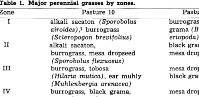
BRANSON ET AL.

Table 1. Classificafion sysfem for vegefafion of the Greaf Basin proposed

by H. L. Shanfz (1925). _{-___}

Northern Desert Shrub Formation

Sagebrush association (Artemisia tridentata) Small sagebrush association (Artemisia nova)

Little rabbitbrush associes (Chrysothamnus puberulus) Shadscale association (Atriplex conjertijolia)

Winterfat associes (Eurotia Zanata)

Hop-sage and Coleogyne association (Grayia spinosa

and

Coleogyne ramosissima)

Bud sagebrush association (Artemisia spinescens) Mat saltbush association (Atriplex corrugata) Gray molly association (Kochia vestita) Salt Desert Shrub (Greasewood) Formation

Greasewood association (Sarcobatus vermiculatus) Greasewood shadscale association (S. vermiculatus

and

Atriplex conjertijolia)

Seepweed association (Dondia torreyana) Pickleweed association (AZZenroZjea occidentalis) Samphire association (Salicorniu utahensis and S. rubra) Saltgrass associes (Distichlis stricta)

Alkali sacaton associes (Sporobolus airoides) Rabbitbrush associes (Chrysothamnus graveolens)

Table 2. Shreve’s (1942) classificafion of Greaf Basin Deserf vegefafion. Juniperus utahensis (6,000 to 7,000 ft)

Artemisia tridentata (upper belt) Atriplex conjertijolia (lower belt) Kochia vestita

Sarcobatus vermiculatus

Distichlis stricta-Sporobolus airoides

Salicornia rubra, S. utahensis, AZZenroZjea occidentalis Coleog yne ramosissima

views that now seems erroneous.

For example, winterfat commu-

nities are now being invaded by

Halogeton glomeratus

(Eckert,

1954); and Fautin (1964) proposed

that much of the type had been

replaced by little rabbitbrush

(Chrysothamnus stenophyllus).

T h e Clemensian terminology

(Weaver and Clements, 1938) oc-

curs infrequently in recent pa-

pers.

Shreve (1942), in his Botanical

Review article on North Ameri-

can deserts, used both the zona-

tion concept and edaphic factors

in his ordination of plant com-

munities (Table 2). However,

Shreve questioned the view that

there are “fundamental units” of

vegetation and recognized that

even

when multiple criteria are

used it is difficult to classify veg-

etation types. Shreve cites the

work by

Kearney and collabora-

tors (1914) and lists their values

for salt tolerances of the species

Table 3. Bio-ecologic classificafion of Greaf Basin vegefafion by Fau- fin (1946).

Finon-Juniper Biome

Northern Desert Shrub Biome Shadscale Community Tetradymia Community Greasewood Community Winterfat Community Black Sage Community Pickleweed Community Little Rabbitbrush Associes Sagebrush Community Southern Desert Shrub Biome

present near the Great Salt Lake.

Shreve’s presentation is a gen-

eral description, but the classifi-

cation in Table 2 may be derived

from it.

(12)

SALT DESERT SHRUBS

289

Table 4. The zonafion concepf ap- plied to Great Basin vegetation by Billings (1949).

Sagebrush zone Shadscale zone

Edaphic climaxes in zone: Greasewood

Greasewood-shadscale Pickleweed

Winterfat On dune sands:

Dalea polyadenia- Tetradynia glabrata Chrysothamnus

stenophyllus

importance equal to that of sage-

brush. In fairness to Clements,

it should be noted that Clements

referred to the type as the Sage-

brush Formation

(Atriplex-Atie-

misia)

which indicates some rec-

ognition of the importance of

species of the two most wide-

spread genera. The classification

of Fautin also shows disagree-

ment with Shantz in the rank of

winterfat as a climax community.

A classification a d o p t e d by

many recent authors is that by

Billings (1949; Table 4). Billings,

in contrast to systems used pre-

viously, applied to the G r e a t

Basin flora the zonation concept

as used by Daubenmire (1943) for

flora of the Rocky Mountains.

An interpretation of Billings’ ar-

ticle shows the listing of two ma-

jor zones: (1) Sagebrush is the

upper, wetter one, and (2) Shad-

scale is the lower, dryer one. He

views all the communities within

the shadscale zone as minor eda-

phic climaxes forming a mosaic.

The quantitative data in the pa-

per by Billings is on Nevada veg-

etation with references to the

work by Fautin (1946) for infor-

mation on Utah Great Basin veg-

etation.

Proposed in Table 5 is a new

vegetation classification based on

maximum salt tolerances of com-

munities and on the capacity of

one group, the Salt Marsh Zone,

to exist partially submerged in

water during all or part of the

year. The data are presented in

atmospheres osmotic stress at

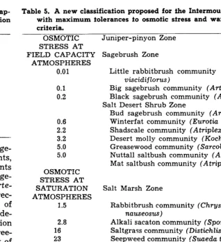
Table 5. A new classification proposed for the Infermounfain shrub region, with maximum iolerances fo osmotic stress and wafer relationships as criteria.

OSMOTIC Juniper-pinyon Zone

STRESS AT FIELD CAPACITY

ATMOSPHERES 0.01 0.1 0.2

0.6 2.2 3.2 5.0 5.0 OSMOTIC STRESS AT SATURATION ATMOSPHERES

1.5 2.8 16 23 35 35 50 75

Sagebrush Zone

Little rabbitbrush community (Chrysothamnus viscidiftorus)

Big sagebrush community (Artemisia tridentata) Black sagebrush community (Artemisia nova) Salt Desert Shrub Zone

Bud sagebrush community (Artemisiu spinescens) Winterfat community (Euro,tia Zunuta)

Shadscale community (AtripZea: confertifolia) Desert molly community (Kochia americanu) Greasewood community (Sarcobatus vermiculatus) Nuttall saltbush community (Atriplex nuttallii) Mat saltbush community (Atriplex corrugata)

Salt Marsh Zone

Rabbitbrush community (Chrysothamnus nauseosus)

Alkali sacaton community (Sporobolus air&ales) Saltgrass community (Distichlis stricta)

Seepweed community (Suuedu torreyana) Glasswort community (Salicornia utahensis

and S. rubra)

Pickleweed community (AZZenroZfea occidentalis) Algae

Fungi

field capacity because of the ease

of interpreting these values in

terms of plant physiology. Max-

imum values for each community

were obtained from published re-

ports and from unpublished data

obtained by the authors. The os-

motic stress at 15 atm soil-mois-

ture stress, the suction force

sometimes considered to be the

permanent wilting point, can be

obtained by multiplying the val-

ues shown by two except for the

Salt Marsh Zone. Osmotic stress

at saturation is shown for Salt

Marsh Zone communities

be-

cause these habitats usually have

moist soils. To obtain total soil

moisture stress for communities

other than those of the Salt

Marsh Zone, the stress associated

with soil-particle size (physical

or matric stress) would be added

to values for osmotic stress.

For all the communities in the

Salt Marsh Zone except rabbit-

brush and alkali sacation, the os-

motic stress alone exceeded the 15

atm sometimes used to represent

the permanent wilting stress. Un-

der conditions that are too salty

for vascular plants in salt marshes

of Death Valley, Hunt (1966)

found algae surviving osmotic

stresses of 50 atm and fungi on

areas with as much as 75 atm.

(13)

290

basin, soil-particle sizes tend to

become smaller as one ap-

proaches the playas, resulting in

higher soil moisture stresses.

Local areas, such as those OCCU-

pied by wind-blown sand and

certain geologic materials, provide exceptions to this general- ization.

The salt marshes that occupy

some playa bottoms are pre-

sented in Table 5 as a separate zone and it should be noted further that these are not true des-

ert plant communities in the

sense that they are limited to

deserts. Salt marshes are also

common in moist climates

(Weaver and Clements, 1938, p. 227) and are even more abundant along seacoasts (Chapman, 1960). Many of the genera and some of the species are the same over much of the world.

Although the maximum os-

motic stress values shown in

Table 5 appear to provide a ra- tional ordination of plant com-

munities, caution must be ap-

plied when using plants as pre- cise indicators of salinity. Gates et al. (1956) found that although mean values differed significant-

ly between communities, there

were overlapping salt tolerances for the five salt desert shrub

communities studied. However,

classif ication of plant communities on the basis of maximum tolerances is in agreement with

the statement by Daubenmire

(1948): “In general, the greater the salt tolerance of a species, the wider the range of salinity of the soils on which it grows, i.e., the degree of maximal salt tolerance is more definite than the minimal.”

Disfribufion of Salf Desert Shrub Communifies

The Great Basin Desert as

mapped by Shreve (1942) extends far beyond the Great Basin phys-

iographic province into the Co-

lumbia Plateau and the upper Colorado River basin. More in-

formation now exists than was

available to Shreve, and the

BRANSON ET AL.

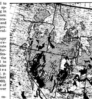
FIG. 1. Distribution of the saltbush-greasewood type (in solid black) and the sagebrush type (cross-hatched). (Revised from Kuchler, 1%4).

boundaries could be extended to include a larger portion of Wy- oming, parts of Montana and a larger portion of New Mexico and still comply with Shreve’s

criteria which emphasized life

forms, structure, and florist&. Shreve’s map indicates the extent of plant communities listed in Table 5. Shreve characterizes the Great Basin Desert as being (4 _{. . .}_{largely above 4,000 ft. and} has frequent periods of freezing temperatures of a week or more in duration.” This contrasts with the Mojave Desert to the south which is largely below 4,500 ft. and is warmer and dryer. A major criterion used by Shreve to separate the two deserts is the presence of creosote bush (Laa- rea trident&a) in the Mojave Desert.

Undoubtedly the best vegeta-

tion map of the United States available at present is the one by Kiichler (1964). Shown in Fig. 1 are tracings from Kiichler’s map with the addition of some salt desert shrub areas in Mon-

tana and Wyoming. The cross-

hatched area represents the types where big sagebrush is dominant and has a planimetered area of 143 million acres, a larger area than some of the estimates that are in print (U.S. Dept. Agr., 1936). The extent of sagebrush types is shown because salt desert shrubs, at least in minor amounts, occur throughout most of the area occupied by big sagebrush.

(14)

SALT DESERT SHRUBS

FIG. 2. Approximate geographic distribution of winterfat (Eurotia lanata), g-reasewood (Sarcobatus vermiculatus), shadscale (Atriplex confertifolia), nuttall saltbush (A. nuttallii), and bud sagebrush (Artemisia spinescens).

many of the estimates in the lit- erature (Hutchings and Stewart, 1953). The three small areas in Montana and one in northeastern

Wyoming are not shown on

Kuchler’s map. Although small,

these areas are important be-

cause the sparse plant cover and fine-textured soils give rise to high sediment y i e 1 d s and, in some areas, spectacular erosion. An example of the latter is the

Willow Creek valley in north-

eastern Montana which has an eroded trench about 20 ft. deep and 30 miles long. Much of the

trenching has occurred during

the life of residents of the area. The basin has been thoroughly treated by the U.S. Bureau of Land Management to control erosion.

Geographic Disfribufion of Salf Desert Shrub ‘Species

The distribution of salt desert shrub species is far greater than

the areas dominated by these

plants (compare Fig. 1 with Fig. 2). The wide latitudinal and lon- gitudinal ranges of these species indicate that some factor or factors other than climate determine

areas in which salt desert shrubs

are dominants. Edaphic factors

seem to determine the presence of pure stands of salt desert shrubs but, as pointed out earlier, many species have overlapping tolerances for soil characteristics

that have been measured. This

view of climatic effects is not

in full agreement with that of

Billings (1949) who states that “The shadscale zone is character-

291

ized by a much dryer climate than the sagebrush zone and lies between the sagebrush and creo- sotebush zones.” The complexity of the problem “Why do plants grow where they do?” has been

thoroughly explored by Billings

(1953). It is hazardous and pos-

sibly erroneous to attempt to

over-simplify the cause and effect relationships responsible for plant species distribution.

Throughout the distributions

shown, salt desert shrubs exert

dominance locally, but usually

on areas too small to appear even on large scale vegetation maps.

However, extensive and nearly

pure stands are largely restricted to the states of Nevada and Utah. The most widely distributed of the salt desert shrubs is winterfat. The wide ecologic amplitude of winterfat is demonstrated by both the extensive geographic area in which it occurs and the variety of species with which it is associated. Altitudinal range

of winterfat is from 2,000 to

10,000 ft.

Greasewood, nuttall saltbush,

and shadscale are almost as

widely distributed as winterfat. There is no apparent reason for the disjunct distribution of shadscale in western Colorado, where it is common, and the isolated area of shadscale in southeastern Colorado.

There are a number of salt tolerant shrubs in the M o j a v e,

Sonoran, and Chihuahuan Des-

erts, but these have not been included in the Salt Desert Shrub Zone of the Great Basin desert.

Although absent or rare in the

Great Basin desert, they merit a brief mention here. Cattle spin- ach (Atriplex poZycarpa) is one of the most important saltbushes in the Sonoran and Mojave des-

erts. Soils occupied by it are

(15)

292

tolerant plants of the southwest deserts. In Death Valley (Hunt, 1966) it occupies “. . . the lowest,

smoothest, saltiest, and hottest parts of the gravel fans.”

One of the most widely distributed saltbushes is four-wing

saltbush (Atriplex canescens).

Although its latitudinal range is from Montana to Mexico it is seldom found in pure stands.

Four-winged saltbush ususally

occurs on sandy soils.

Some causafive factors for the presence of salt desert

shrub communities

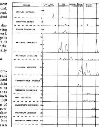
Shown on Fig. 3 are plant communities as found on different strata of Bearpaw Shale exposed on a hill in Montana. The data shown are hits per 100 pins as measured by the all contacts

point-quadrat method at Z-inch

intervals over a distance of 1,080 ft from the top to the bottom of the hill. The Curtiss (1956) con- tinuum concept or the Whittaker (1953) population pattern concept could be applied to the data, but the classical concept (H a n s o n and Churchill, 1961) which recog- nizes dominance and names com-

munities seems preferable. Nut-

tall saltbush communities are

present on the dry, exposed hilltop and again on fine-textured alluvium at the base of the hill. Big sagebrush types occur adjacent to the two nuttall saltbush types. Centrally located on the hill in a highly gypsiferous soil is a buckwheat (Eriogonum mul-

ticeps) community. Two species

showing wide ecologic amplitude

are western wheatgrass (Agropy-

ran smithii) and knotweed (Poly- gonum aviculure). It is probable that propagules from species of

each plant community have

reached all the habitats on the

hill almost annually, but the

communities remain distinct.

This statement leads to the very difficult question, ‘

‘W

h y a r e

these adjacent plant communities different?”

This report seems to us to re-

quire some brevity, thus only

BRANSON ET AL.

AGROPYRON SMlTHll

OPUNTIA POLYCANTHA

ARTEMISIA TRIDENTATA

_PO”“O”“_AV~““E_ ‘;t ( ,., ,mbj,\ .

TtlERMOPSIS RHOMBIFOLIA

---

_O1

ROSA ARKANSANA _lot

_---_---0

CALAHOVILFA LONGIFOLIA

ROCK

---D FEET DOWNHILL

MIXED SHRUBS

_ ?.. .

AL

i. .

dt,

,...*, ‘4, .._,. \,

,f.\.

,. . .

J -I-.!_.. 600

FIG. 3. Plant communities on a hill with different strata of Bearpaw Shale exposed. The data are hits per 100 pins, as determined by the all contacts point-quadrat method with pins at two-inch intervals.

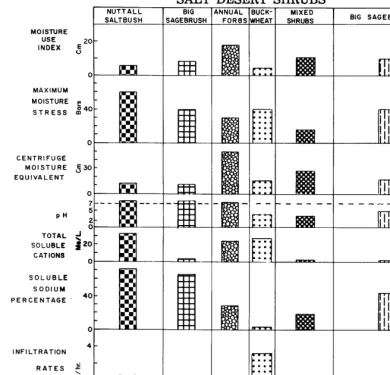
the highlights of Fig. 4 will be discussed. The moisture use in-

dex (differences between maxi-

mum and minimum storage cal- culated in cc) is low for the two nuttall saltbush communities, and maximum total soil-moisture stress reached near the depth to

which roots penetrated was

greatest in these two communities. These data show that nuttall saltbush is the most drought tolerant of the species present on the sampling sites. Centrifuge moisture equivalents, represent- ing moisture storage possible at field capacity to the depth of rooting, are similar to, but ex-

ceed, the moisture-use index.

These are expected results be-

cause field capacity percentages were seldom reached in the soils studied. pH has no apparent effect on the plant community differences. The high pH at the top of the hill is caused by an out- crop of limestone, indicated as rock at the bottom of Fig. 3. Total soluble cations are highest in soils of the two nuttall saltbush communities indicating that this species is salt tolerant as well as drought tolerant. As has been found in many other studies (Gates et al, 1956; Fireman and

(16)

SALT DESERT SHRUBS 293

MOISTURE

USE 20

INDEX 5

0

MAXIMUM MOISTURE L1

STRESS t%i4’

0

CENTRIFUGE

MOISTURE 530

EQUIVALENT

0 7

PH 5

TOTAL 2

SOLUBLE 3 20 CATIONS

0

SOLUBLE SODIUM

PERCENTAGE 40

0

4 INFILTRATION

RATES 5

: 2

FEET 0 200

B1G

SAGEBRUSH

MIXED

SHRUBS BIG SAGEBRUSH

FIG. 4. Physical and chemical characteristics of soils for the seven plant communities shown in Fig. 3.

occupied sites that contained low quantities of salts.

The soils of the nuttall saltbush communities were sod i c and, surprisingly, the two big sagebrush communities were also present on soils containing high soluble sodium percentages. Gates et al. (1951) found big sagebrush on soils with low sodium values. Soils of the buckwheat type had low sodium contents, but relatively high quantities of salts. This provides evidence that the primary cation in the soils occupied by buckwheat is calcium and additional evidence is provided by the presence of gypsum crystals, selenite, on the soil surface.

Infiltration rates as measured by a portable infiltrometer (Mc- Queen, 1963) gave variable re-

sults that do not appear directly related to soil moisture measurements. All rates were low and only one, the buckwheat, had a rate exceeding one inch (2.54 cm)/ hr. The infiltrometer has measured rates of up to nearly 14 inches/hr. on sandy soils in Cali- fornia (Branson et al., 1961).

From these data it is concluded that soil-moisture relationships are the primary cause of the different plant communities. Quan- tities of soil salts also appear to be important as a cause of community differences, but it may be that the major effects of salts is their osmotic stress contribu- tion to total soil-moisture stress. The only community of the seven that may be present as a result of kinds of soil chemicals is the buckwheat type which occurred on gypsiferous soil.

(17)

294 BRANSON ET AL.

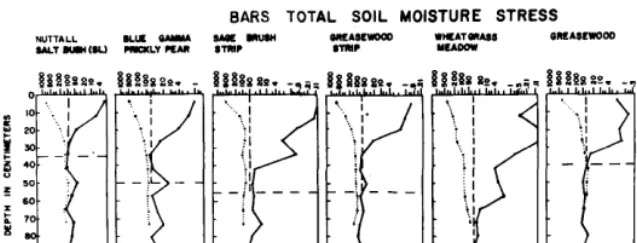
BARS TOTAL SOIL MOISTURE STRESS

NUTTILL KUOYYIsMcmuw _%iF= WIKATSRASS QMASLWQOO SILVER

SMlIu((SLl mcRLY Pun SYMC YKAmW miot-

t

PERCENT MOISTURE IN FILTER PAPERS

FIG. 5. Minimum total soil moisture stress for the season is represented by the solid line, maximum stress by the dotted line, and average maximum stress attained by each community is shown by the vertical dashed line. The data are for 7 plant com- munities in the Willow Creek basin in northeastern Montana.

when related to the kinds of plants growing on the different soils. One interpretation is that the average total soil-moisture stress at this depth represents the maximum stress to which the plants present on each site can remove moisture from the soil. Stresses greater than this average are attributable to water re- moved from the soils by solar energy. Of the com’munities shown, nuttall saltbush had the smallest quantity of plant material to intercept solar radiation and the highest moisture stress near the soil surface, whereas the quantity of plant material was greatest in the silver sagebrush community which had the lowest total soil-moisture stress at the average rooting depth. Average total soil-moisture stress was more than 90 bars for the nuttall saltbush soil and 35 bars for the silver sagebrush sdil. These data were derived from a new calibration of filter paper moisture as a measure of total soil moisture stress and differ somewhat from the values shown in Fig. 4. Analysis of variance for these data shows that differences between the seven communities are highly significant.

The data on average total soil moisture stress can be more easi- ly compared in Fig. 6 than in Fig. 5. The range of values for the 14 plant communities is from more than 90 bars for nuttall saltbush to only 19 bars for the

mixed shrub community. To one familiar with the habitat re- quirements of the species shown, the grouping appears logical. One possible exception is the low drought tolerance indicated for the greasewood-western wheatgrass type. A possible explanation of this seeming discrepancy

is that soil moisture sampling was to a depth of three ft, but greasewood is known to have roots extending to more than 19 ft in the area studied.

Measurements of osmotic stress do not show that halo- phytes occupy only soils high in salts (Fig. 7). Data shown in Fig. 7 were obtained as a part of a study of mechanical treatment effects (Branson et al., 1966) in Montana, Wyoming, Utah, Colo- rado, Arizona, and New Mexico. Although the criterion for site selection was the presence of mechanically treated land, a variety of vegetation types were included in the 58 areas sampled. Barren ground and nuttall saltbush occupied the sites highest in salts, but other halophytic types such as nuttall saltbush- blue grama, shadscale, spiny horsebrush, and winterfat, were

AVERAGE MAXIMUM TOTAL SOIL MOISTURE STRESS( Bars)

0 IO 20 30 40 50 60 70 so 90

NUTTALLSALTBUSH SLICK

NUT-TALL SALTBUSH HILLTOP

NUllAlL SALTBJSH SOYI-SLICK

GREASEwOoDSTmP

BIG SAGE-PRICKLYPEAR

BIG SEBRUSH STRIP

BIG SAGEBRUSH

GREASEWOOD-WESTERN WHEATGRASS

BLUEGRAMA

SlLVER SAGEBRUSH-WESTERNWHEATGRASS