Community Intercomparison Suite (CIS) v1.4.0: a tool for intercomparing models and observations

(1)

doi:10.5194/gmd-9-3093-2016

Community Intercomparison Suite (CIS) v1.4.0: a tool for

intercomparing models and observations

Duncan Watson-Parris1,2_{, Nick Schutgens}2_{, Nicholas Cook}1_{, Zak Kipling}2_{, Philip Kershaw}3,4_{, Edward Gryspeerdt}5_, Bryan Lawrence3,6,7_{, and Philip Stier}2

1_{Tessella Ltd, Abingdon, Oxford, UK}

2_{Atmospheric, Oceanic and Planetary Physics, Department of Physics, University of Oxford, Oxford, UK} 3_{Centre for Environmental Data Analysis, STFC Rutherford Appleton Laboratory, Didcot, UK}

4_{National Centre for Earth Observation, Leicester, UK}

5_{Institute for Meteorology, Universität Leipzig, Leipzig, Germany} 6_{Department of Meteorology, University of Reading, Reading, UK} 7_{National Centre for Atmospheric Science, Leeds, UK}

Correspondence to:Duncan Watson-Parris ([email protected]) Received: 4 February 2016 – Published in Geosci. Model Dev. Discuss.: 15 March 2016 Revised: 11 August 2016 – Accepted: 15 August 2016 – Published: 6 September 2016

Abstract. The Community Intercomparison Suite (CIS) is an easy-to-use command-line tool which has been devel-oped to allow the straightforward intercomparison of re-mote sensing, in situ and model data. While there are a number of tools available for working with climate model data, the large diversity of sources (and formats) of remote sensing and in situ measurements necessitated a novel soft-ware solution. Developed by a professional softsoft-ware com-pany, CIS supports a large number of gridded and ungrid-ded data sources “out-of-the-box”, including climate model output in NetCDF or the UK Met Office pp file format, CloudSat, CALIOP (Cloud-Aerosol Lidar with Orthogonal Polarization), MODIS (MODerate resolution Imaging Spec-troradiometer), Cloud and Aerosol CCI (Climate Change Ini-tiative) level 2 satellite data and a number of in situ air-craft and ground station data sets. The open-source architec-ture also supports user-defined plugins to allow many other sources to be easily added. Many of the key operations re-quired when comparing heterogenous data sets are provided by CIS, including subsetting, aggregating, collocating and plotting the data. Output data are written to CF-compliant NetCDF files to ensure interoperability with other tools and systems. The latest documentation, including a user manual and installation instructions, can be found on our website (http://cistools.net). Here, we describe the need which this tool fulfils, followed by descriptions of its main functionality

(as at version 1.4.0) and plugin architecture which make it unique in the field.

1 Introduction

Modern global climate models (GCMs) produce huge amounts of prognostic and diagnostic data covering every aspect of the system being modelled. The upcoming CMIP6 (Coupled Model Intercomparison Project Phase 6) is likely to produce as much as 40 Pb of data alone (Eyring et al., 2016a). Analysis of the data from these models forms the corner-stone of the IPCC (Stocker et al., 2013) (Intergovernmental Panel on Climate Change) and subsequent UNFCCC (United Nations Framework Convention on Climate Change) reports on anthropogenic climate change, but there exist large dif-ferences across the models in a number of key climate vari-ables (e.g. Boucher et al., 2013; Suzuki et al., 2011). In or-der to unor-derstand these differences and improve the models, the model data must be compared not only with each other – which is relatively straightforward for large intercompari-son projects, such as CMIP, which provide the model data in a common data standard – but also with observational data, which can be much harder.

(2)

eas-ily produce petabytes of data over their lifetime. There are dozens of EO satellites being operated by the National Aero-nautics and Space Administration (NASA), the European Space Agency (ESA) and other international space agencies. While modern missions use common data standards, there are many valuable data sets stored in unique formats and structures which were designed when storage was at more of a premium, and so are not particularly user-friendly. Ground-based EO sites and in situ measurement of atmospheric prop-erties are also areas where many different groups and organi-zations produce data in a wide variety of formats.

The process of model evaluation typically involves a rel-atively small set of common operations on the data: read-ing, subsettread-ing, aggregatread-ing, analysis and plotting. Many of these operations are currently written as a bespoke analy-sis for each type of data being compared. This is time con-suming and error prone. While a number of tools currently support the comparison and analysis of model data in stan-dard formats, such as NetCDF Operators (NCO) (Zender, 2008), Climate Data Operators (CDO) (http://www.mpimet. mpg.de/cdo), Iris (Met Office, 2016) and CF-Python (http: //cfpython.bitbucket.org) there are few, if any, which sup-port raw observational data. A tool described by Langerock et al. (2015) provides some of this functionality for a specific set of observational data, ESMValTool provides a framework for comparison against standardized observations (Eyring et al., 2016b) and Program for Climate Model Diagnosis and Intercomparison (PCMDI) Metrics Package (PMP) pro-vides some comparisons with globally averaged observa-tions (Gleckler et al., 2016). There are also some websites which allow a pre-defined analysis of specific data sets (for example, Giovani: http://giovanni.sci.gsfc.nasa.gov), but do not give the flexibility of a tool which can be installed and run locally. The Community Intercomparison Suite (CIS) seeks to fill this gap: the primary goal of CIS is to provide a single, flexible tool for the quantitative and qualitative intercompar-ison of remote-sensing, in situ and model data.

Comparing global model data with observations that can be considered point measurements may introduce substan-tial errors in any analysis (Schutgens et al., 2016a). Aggre-gation of observations may reduce these errors and facili-tate intercomparisons of model data and (now gridded) ob-servations (see Appendix A for a definition of “aggregated data” and other terms). Aggregated observational data are often available (e.g. from the Obs4MIPs project, Teixeira et al., 2014). However, errors may be introduced through sub-optimal aggregation procedures, when using sparse data sets (Levy et al., 2009) or when aggregating over long time periods (Schutgens et al., 2016b). A comparison of data that are most similar in their spatio-temporal sampling can be shown to provide improved confidence when constraining aerosol processes in climate models (Kipling et al., 2013). Thus, there is a need for a flexible aggregation and collo-cation tool for both gridded and ungridded data that allows

straightforward point-wise comparison between a variety of data formats.

In this paper, we first describe the development of this new tool (Sect. 2) and the architecture designed to allow maxi-mum flexibility in the data types and functionality supported (Sect. 3). Then, tables of the specific types of data CIS sup-ports and detailed descriptions of the operations which can be performed on them are provided (Sect. 4), followed by an example of the scientific workflow which this tool enables (Sect. 5). Information about downloading and installing CIS or accessing the source code can be found in Sect. 7. A brief description of the plugin architecture and the steps needed for a user to create their own plugins are provided in Ap-pendix B and a table of definitions in ApAp-pendix A. A refer-ence card providing a one-page summary of the various CIS commands is also available as a supplement to this paper.

2 Development

CIS has been developed by a professional software devel-opment consultancy (Tessella Ltd.) working closely with the Centre for Environmental Data Analysis (CEDA) and the De-partment of Physics at the University of Oxford to ensure a high quality tool which meets the need of a broad range of users. The use of modern development practices such as test-driven development (TDD) (Beck, 2003) and continuous in-tegration (CI) (Beck, 2000) has ensured that each component is automatically tested against hundreds of unit tests before it is deployed. These test each individual function within the code to ensure defects are kept to a minimum and particu-larly reduce regressions (defects introduced into code which was previously working).

The development was also carried out in an agile fashion, specifically using Scrum (Schwaber and Beedle, 2001). In this approach, regular working releases were made at the end of 2-week implementation “sprints”, each delivering a priori-tized set of fully functioning requirements adding immediate value to the users (scientists). The developers were supported by a subject matter expert (SME) who worked with the scien-tists to define and prioritize each area of development (user stories), a dedicated testing specialist who was responsible for defining and performing independent testing and a project manager (PM) who oversaw progress and managed the over-all development process from the Tessella perspective.

(3)

Much consideration was given to the need for paralleliza-tion and optimizaparalleliza-tion of the funcparalleliza-tions within CIS, particu-larly around collocation where long runtimes for large data sets can be expected. Significant development time was de-voted to optimizations in these functions and many of the runtimes now scale very well with size of the data. However, we deemed it a lower priority to devote development time to parallelizing these operations, as they are usually trivially parallelized by the user by performing the operation on each input file separately across the available compute nodes (us-ing a batch script, for example, and subsett(us-ing the data first as needed). Such a script is pre-installed alongside CIS on the UK JASMIN big-data analysis cluster (Lawrence et al., 2012) and could be easily ported to other clusters.

All of the source code for CIS is freely available under the GNU Lesser General Public License v3, which is expected to promote widespread uptake of the tool and also encourage wider collaboration in its development.

3 Extensible architecture

One of the key features of CIS is the flexible and extensible architecture. From the outset it was obvious that there was no way for a single, unextendable, tool to provide compatibility with the wide variety of data sources available and support all of the various analyses which would be performed on them. A modular design was therefore incorporated, which allowed user-defined components to be swapped in as easily as pos-sible.

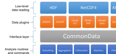
At the heart of the design is the CommonData interface layer which allows each of the analysis routines and com-mands to work independently of the actual data being pro-vided, as shown in Fig. 1. The top row of modules in this fig-ure represents the low-level reading routines which are used for actually reading and writing data to the different data for-mats. The orange components are the data products which interpret the data for CIS and can be swapped out by the user (using plugins, as described in Sect. B1). The CommonData block represents the internal CIS data structure which ab-stracts the CIS functionality (shown in the bottom row) from the different data formats above. Specifically, CommonData is an abstract base class (a class defines an object in object oriented programming) which defines a number of methods which the analysis routines can assume will exist regardless of the underlying data. The two main concrete types of Com-monData are GriddedData and UngriddedData, which repre-sent gridded and ungridded data, respectively.

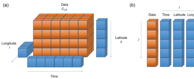
There are an extensive number of data sources which are supported by CIS, which can be broadly categorized as ei-ther gridded or ungridded data. Gridded data are defined as any regularly gridded data set for which points can be in-dexed using(i, j, k, . . .)wherei,j andkare integer indexes on a set of orthogonal coordinates (see Fig. 2a). Here we define the gridded data values as an n-dimensional matrix

Figure 1.An illustration of the architecture of CIS demonstrating the different components in the modular design.

Gandncoordinate vectors x,y, . . ., which we will use in the algorithmic descriptions of the operations in Sect. 4. Un-gridded data are anything which does not meet this criteria and, in general, it is assumed each(x, y, z)point is indepen-dent of every other point (Fig. 2b). Then, we can define a data valueujand set of coordinatesrj at each pointj. Note that although this independence may not strictly be true for some of the data sources (for example, satellite mounted li-dar instruments where many altitude points will be present for each latitude/longitude point) this strict definition applies within CIS. This allows significant optimizations to be made for operations on gridded data and flexibility in dealing with ungridded data, at the expense of performance for some op-erations on those ungridded data sets which do have some structure.

In CIS, the gridded data type is really just a thin wrapper around the cube provided by the Iris (Met Office, 2016) li-brary. All of the ungridded routines are however bespoke and include a number of useful features (besides the main anal-ysis routines) including multi-file and multi-variable opera-tions, hierarchical NetCDF file reading and automatic recog-nition of file types. The ungridded data are stored internally as one NumPy (van der Walt et al., 2011) array of values and a set of associated metadata. There is one such structure for the data values themselves and each of the latitude, lon-gitude, time and altitude coordinates (as needed). The data array may take on any shape but all of the corresponding co-ordinate arrays (lat, long, etc. as shown in Fig. 2b) must have the same shape.

4 Core functionality

In this section, we describe the core functionality of CIS. Each sub-section gives a brief description of an operation, the command line syntax and expected output, a formal al-gorithmic description of the operation (where appropriate) and a short example.

(4)

Figure 2. (a)An illustration of the design of the gridded data objects used internally by CIS – based heavily on the Iris cube. Then

-dimensional data arrayGis accompanied bynone-dimensional coordinate arrays. Note that hybrid height and pressure coordinates can also

be created and used as needed.(b)An illustration of the design of ungridded data objects used internally by CIS. Alljpoints are assumed to

be independent of each other. The data and associated coordinates are represented as a series of one-dimensional arrays.

to define vector inequalities as

ifx5ythenxi≤yi for alli=1, . . ., n, (1) where≤is the standard (single-value) inequality and we ap-ply it here to all values in the vector; similar identities can be defined for the other inequalities. We use∅to denote an empty set,∀should be read as “for all”,:as “such that” and∨ as logical “and”. Some operations involve the use of a kernel to reduce a set to a single value, we denote these asK.

Although data reading is something a user is rarely aware of when using CIS, the flexibility offered in this regard is an important distinguishing feature. All of the functions de-scribed in the following sections are possible with any of the supported data sets and any data sets supported by user-written plugins (as described in Sect. B1).

A list of the ungridded data sources supported by CIS out-of-the-box is presented in Table 1 and grid-ded data sources in Table 2. As CIS uses Iris for gridded data support, any climate and forecast (CF) compliant (http://cfconventions.org/Data/cf-conventions/ cf-conventions-1.6/build/cf-conventions.pdf) NetCDF4 data can be read in with CIS, as well as the other formats listed.

For all supported data sets any missing_value and

_FillValue attributes (or the equivalent for that data

set) are automatically taken into account, as well as any

valid_min,valid_maxandvalid_rangeattributes

to mask out invalid data values. Scaling factors and offsets are also applied as appropriate for each data set.

4.1 Subsetting

Subsetting allows the reduction of data by extracting vari-ables and restricting them to user-specified ranges in one or more coordinates. Both gridded and ungridded data sets can be reduced in size by specifying the range over which the output data should be included, and points outside that range are removed.

The basic structure of the subset command is

$ cis subset <datagroup> <limits> [-o output_file]

where “subset” is the sub-command to invoke in “cis” and the “output_file” is the (optional) filename to be used for out-putting the result. If none is specified then a default is used. The two main arguments “datagroup” and “limits” are more complex and will be discussed below.

The datagroup is a common concept across the various CIS commands. It represents a collection of variables (from a collection of files) sharing the same spatio-temporal coor-dinates, which takes the form

variables:filenames[:product=...]

Here, the “variables” element specifies the variables to be operated on and can be a single variable, a comma-separated list, a wildcarded variable name or any combination thereof. The “filenames” element specifies the files to read the vari-ables from and can be a single filename, a directory of files to read, a comma-separated list of files or directories, wild-carded filenames or any combination thereof. The optional “product” element can be used to manually specify the par-ticular product to use for reading this collection of data. See Tables 1 and 2 for a full list of initially available product names.

The “limits” are a comma-separated list of the upper and lower bounds to be applied to specific dimensions of the data. The dimensions may be identified using their variable names (e.g. latitude) or by choosing a shorthand from “x”, “y”, “z”, “p” or “t” which refer to longitude, latitude, altitude, pressure and time, respectively. The limits are then defined simply using square brackets, e.g. x= [−10,10]. The use of square brackets is a useful reminder that the intervals are inclusive, as discussed below. A time dimension can be specified as an explicit window

(5)

Table 1.A list of the ungridded data sources supported by CIS 1.4.0. The file signature is used by CIS to automatically determine the correct product to use for reading a particular set of data files, although this can easily be overridden by the user. (Internally these signatures are represented as Python regular expressions; here, they are shown as standard wildcards for ease of reading.). The Global Aerosol Synthesis and Science Project (GASSP) data sets are large collections of harmonized in situ aerosol observations from groups around the world (http://gassp.org.uk).

Data set Product name Type File signature

MODIS L2 MODIS_L2 Satellite *MYD06_L2*.hdf, *MOD06_L2*.hdf, *MYD04_L2*.hdf,

*MOD04_L2*.hdf, *MYDATML2.*.hdf, *MODATML2*.hdf

Aerosol CCI Aerosol_CCI Satellite *ESACCI*AEROSOL*

Cloud CCI Cloud_CCI Satellite *ESACCI*CLOUD*

CALIOP L1 Caliop_L1 Satellite CAL_LID_L1-ValStage1-V3*.hdf

CALIOP L2 Caliop_L2 Satellite CAL_LID_L2_05kmAPro-Prov-V3*.hdf

CloudSat CloudSat Satellite *_CS_*GRANULE*.hdf

NCAR-RAF NCAR_NetCDF_RAF Aircraft *.nc containing the attribute Conventions with the value

NCAR-RAF/nimbus

GASSP NCAR_NetCDF_RAF Aircraft *.nc containing the attribute GASSP_Version

GASSP NCAR_NetCDF_RAF Ship *.nc containing the attribute GASSP_Version, with no altitude

GASSP NCAR_NetCDF_RAF Ground station *.nc containing the attribute GASSP_Version, with attributes

Sta-tion_Lat, Station_Lon and Station_Altitude

AERONET AERONET Ground stations *.lev20

CSV data points ASCII_Hyperpoints N/A *.txt

CIS ungridded cis CIS output *.nc containing a source attribute which starts with “CIS”

Table 2.A list of the gridded data sources supported by CIS 1.4.0. The file signature is used by CIS to automatically determine the correct product to use for reading a particular set of data files. This can always be overridden by the user.

Data set Product name Type File signature Net_CDF Gridded Data NetCDF_Gridded Any

CF-NetCDF4-compliant gridded data

*.nc (this is the default for NetCDF Files that do not match any other signature)

MODIS L3 daily and 8 day MODIS_L3 Satellite *MYD08_D3*.hdf, *MOD08_D3*.hdf, *MOD08_E3*.hdf UK Met Office pp data HadGEM_PP Gridded model data *.pp

or more simply as a single value: t=[2010]. In this case,

the value is interpreted as both the start and the end of the window and all points which fall within 2010 would be included. For all other dimensions, the values are compared directly with those from the data file (although these can be converted to standard units during reading if required).

The detailed algorithm used for subsetting ungridded data is outlined in Algorithm 1 and for gridded data in Algo-rithm 2. The algoAlgo-rithms use a mix of pseudo-code and mathe-matical notation to try to present the operations in a clear but accurate way. The operations themselves will involve other checks and optimizations not shown in the algorithms, but the code is available for those interested in its exact work-ings. See Sect. 3 for definitions of the gridded and ungridded entities.

For example, the following command would take the vari-able “aod550” from the file “satellite_data.hdf”

and output the data contained in a lat/long region around North America for the 4 February 2010 to a file called

“subset_of_satelite_data.nc”:

$ cis subset aod550:satellite_data.hdf x=[-170,-60],y=[30,85],t=[2010-02-04] -o subset_of_satelite_data

The output file is stored as a CF-compliant NetCDF4 file. 4.2 Aggregation

CIS also has the ability to aggregate both gridded and ungrid-ded data along one or more coordinates. For example, it can aggregate a model data set over the longitude coordinate to produce a zonal mean or aggregate satellite imager data onto a 5◦_{lat/long grid.}

The aggregation command has the following syntax:

$ cis aggregate <datagroup>[:options] <grid> [-o outputfile]

(6)

3098 D. Watson-Parris et al.: Community Intercomparison Suite (CIS)

18 D. Watson-Parris et al.: Community Intercomparison Suite (CIS)

Stocker, T. F., Qin, D., Plattner, G. K., Tignor, M., Allen, S. K., Boschung, J., Nauels, A., Xia, Y., Bex, V., and Midgley, P. M. (Eds.): Climate Change 2013: The Physical Science Basis. Con-tribution of Working Group I to the Fifth Assessment Report of the Intergovernmental Panel on Climate Change, Cambridge

5

University Press, Cambridge, United Kingdom and New York, NY, USA, 2013.

Suzuki, K., Stephens, G. L., van den Heever, S. C., and Nakajima, T. Y.: Diagnosis of the Warm Rain Process in Cloud-Resolving Models Using Joint CloudSat and MODIS Observations, J.

At-10

mos. Sci., 68, 2655–2670, 2011.

Teixeira, J., Waliser, D., Ferraro, R., Gleckler, P., Lee, T., and Potter, G.: Satellite Observations for CMIP5: The Gene-sis of Obs4MIPs, Vol. 95, American Meteorological Society, 2014.TS11

15

van der Walt, S., Colbert, S. C., and Varoquaux, G.: The NumPy Ar-ray: A Structure for Efficient Numerical Computation, Comput. Sci. Eng., 13, 22–30, 2011.

Watson-Parris, D., Schutgens, N. A. J., Cook, N., Kipling, Z., Ker-shaw, P., Gryspeerdt, E., Stier, P., and Lawrence, B.: CIS: v1.4.0, 20

doi:10.5281/zenodo.59939, 2016.TS12

Zender, C. S.: Analysis of self-describing gridded geoscience data with netCDF Operators (NCO), Environ. Model. Softw., 23, 1338–1342, 2008.

Algorithm 1Subset an ungridded dataset given lower and

upper bounds (aandbrespectively) and return the subset as

o.

INITIALIZEo= ∅ forj=1,...,Jdo

oj=ujifa5rj5b end for

Algorithm 2Subsetting a gridded datasetG. Here we de-fine the algorithm for a two-dimensional dataset, although it can trivially be extended to higher dimensions. Given lower

and upper bounds,aandbrespectively for each dimension,

return the subset asO.

ifcells have upper and lower boundsxuandxlrespectivelythen O= {Gij∀i, j:(ax≤x_iu∨x_il≤bx)∨(ay≤y_ju∨y_jl≤by)} else

O= {Gij∀i, j:(ax≤xi≤bx)∨(ay≤yj≤by)} end if

Algorithm 3The ‘box’ collocation of an ungridded dataset

onto a sampling set of coordinatesskofK points. By

def-inition the outputois defined on the same spatio-temporal

sampling ass. The distance metricsDare defined for each

coordinate and compared with the user defined maximuma

(the edge of the ‘box’).

INITIALIZEo= ∅ fork=1,...,Kdo

Q= {uj∀j:D(sk, rj) <a} ok=K(Q)

end for Please note the remarks at the end of the m anuscript.

Geosci. Model Dev., 9, 1–19, 2016 www.geosci-model-dev.net/9/1/2016/

The optional arguments should be given as

keyword=value pairs in a comma-separated list.

The only currently available option (other than the “product” option described in the datagroup summary above) is the “kernel” option. This allows the user to specify the exact aggregation kernel to use. If not specified, the default is “moments” which returns the number of points in each grid cell, their mean value and the standard deviation in that mean. Other options include “max” and “min” which return the maximum and minimum value in each grid cell, respectively.

The mandatory “grid” argument specifies the coordinates to aggregate over. The detail of this argument and the inter-nal algorithms applied in each case are quite different when dealing with gridded and ungridded data so they will be de-scribed separately below. This difference arises primarily be-cause gridded data can be completely averaged over one or more dimensions and also often require area weights to be taken into account.

4.2.1 Ungridded aggregation

In the case of the aggregation of ungridded data, the manda-tory “grid” argument specifies the structure of the binning to be performed for each coordinate. The user can spec-ify the start, end and step size of those bins in the form

coordinate=[start,end,step]. The step may be

missed, in which case the bin will span the whole range given. Coordinates may be identified using their variable names (e.g. “latitude”) or by choosing from “x”, “y”, “t”, “z”, “p” which refer to longitude, latitude, time, altitude and pres-sure, respectively. Multiple coordinates can be aggregated over, in which case they should be separated by commas.

The output of an aggregation is always regularly gridded data, so CIS does not currently support the aggregation over only some coordinates. If a coordinate is not specified (or is specified, but without a step size) then that coordinate is completely collapsed. That is, we average over its whole range, so that the data are no longer a function of that co-ordinate. Specifically, one of the coordinates of the gridded output would have a length of one, with bounds reflecting the maximum and minimum values of the collapsed coordinate.

The algorithm used for the aggregation of ungridded data is identical to ungridded to gridded collocation (as this is

es-Stocker, T. F., Qin, D., Plattner, G. K., Tignor, M., Allen, S. K., Boschung, J., Nauels, A., Xia, Y., Bex, V., and Midgley, P. M. (Eds.): Climate Change 2013: The Physical Science Basis. Con-tribution of Working Group I to the Fifth Assessment Report of the Intergovernmental Panel on Climate Change, Cambridge

5

At-10

mos. Sci., 68, 2655–2670, 2011.

15

doi:10.5281/zenodo.59939, 2016.TS12

o_.

INITIALIZEo= ∅ forj=1,...,Jdo

Algorithm 2Subsetting a gridded dataset G. Here we de-fine the algorithm for a two-dimensional dataset, although it can trivially be extended to higher dimensions. Given lower

ifcells have upper and lower boundsxuandxlrespectivelythen O= {Gij∀i, j:(ax≤xui ∨xil≤bx)∨(ay≤yju∨yjl ≤by)} else

onto a sampling set of coordinatessk ofK points. By

def-inition the output ois defined on the same spatio-temporal

sampling ass. The distance metrics_Dare defined for each

end for Please note the remarks at the end of the m anuscript.

sentially a collocation operation with the grid defined by the user) described in Algorithm 4.

An example of the aggregation of some satellite data which contain latitude, longitude and time coordinates is shown below. In this case, we explicitly provide a 1◦_×₁◦ latitude and longitude grid and implicitly average over all time values.

$ cis aggregate AOT500:

satellite_data.nc: kernel=mean x=[-180,180,1],y=[-90,90,1] -o agg-out.nc

4.2.2 Gridded aggregation

For gridded data, the binning described above is not currently available; this is partly because there are cases where it is not clear how to apply area weighting. (The user would receive the following error message if they tried: “Aggregation using partial collapse of coordinates is not supported for Gridded-Data”.) The user is able to perform a complete collapse of any coordinate however, simply by providing the name of the coordinate(s) as a comma-separated list; e.g. “x,y” will aggregate data completely over both latitude and longitude, but not any other coordinates present in the file.

The algorithm used for this collapse of gridded di-mensions is more straightforward than that of the ungrid-ded case. First, the area weights for each cell are calcu-lated and then the dimensions to be operated on are av-eraged over simultaneously. That is, the different moments of the data in all collapsed dimensions are calculated to-gether, rather than independently (using the Iris routines described here: http://scitools.org.uk/iris/docs/latest/iris/iris/ cube.html#iris.cube.Cube.collapsed), as values such as the standard deviation are non-commuting.

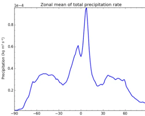
A full example of gridded aggregation, taking the time and zonal average of total precipitation from the HadGEM3 (He-witt et al., 2011) GCM is shown below. A plot of the resulting data is shown in Fig. 3.

(7)

Figure 3.A plot of the zonal average of global rainfall, demonstrat-ing the simple aggregation of global model outputs usdemonstrat-ing CIS. See the text for the exact command used to produce this output.

4.3 Collocation

Point-wise quantitative inter-comparisons require the data to be mapped onto a common set of coordinates before anal-ysis, and CIS provides a number of straightforward ways of doing this. One of the key features of CIS is the ability to collocate one or more arbitrary data sets onto a common set of coordinates, for example, collocating aircraft data onto hybrid-sigma model levels or satellite data with ground sta-tion data. The opsta-tions available during collocasta-tion depend on the types of data being analysed as demonstrated in Table 3. The points which are being mapped on to are referred to as sample points, and the points which are to be mapped are referred to as data points.

The basic structure of the collocation command is

$ cis col <datagroup> <samplegroup> [-o outputfile]

where the datagroup specifies the data variables and files to read as described above. The “samplegroup” is analogous to a datagroup, except in this case the data being specified are that of the sample data, that is, the points which the data should be collocated onto.

The samplegroup has a slightly different format to the datagroup, as the sample variable is optional, and all of the collocation options are specified within this construct. It is of the formatfilename:options. The “filename” is one or

more filenames containing the points to collocate onto. The available options (which should be specified in a comma-separated list) are listed below:

– variable is used to specify which variable’s

coor-dinates to use for collocation. This is useful if a file contains multiple coordinate systems (common in some

model output). Note, that if a variable is specified, miss-ing variable values will not be used as sample points.

– collocator is an optional argument that

spec-ifies the collocation method. Parameters for the collocator, if any, are placed in square brack-ets after the collocator name, for example,

collocator=box[h_sep=1km,a_sep=10m].

Here “h_sep” and “a_sep” are parameters which define the size of the collocation box and stand for horizontal separation and altitude separation, respectively. Full details of all of the available parameters can be found in the documentation. If not specified, a default collocator is identified for the data/sample combination. The collocators available, and the one used by default for each sampling combination of data structures, are laid out in Table 3.

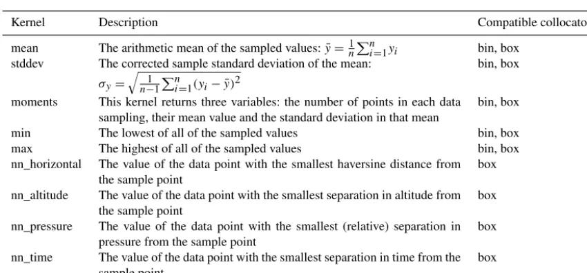
– kernelis used to specify the kernel to use for

colloca-tion methods that create an intermediate set of points for further processing, that is “box” and “bin”. The default kernel in both cases is “moments”. The built-in kernel methods currently available are summarized in Table 4. A full example would be:

$ cis col rain:mydata??.* mysamplefile.nc:collocator= box[h_sep=50km,t_sep=6000S], kernel=nn_t -o my_col

There are also many other options and customizations available. For example, by default all points in the sample data set are used for the mapping. However, (as CIS provides the option of selecting a particular variable as the sampling set) the user is able to disregard all sample points whose val-ues are masked (whose value is equal to the corresponding fill_value). The many different options available for colloca-tion, and each collocator can be found in the user manual (see http://cis.readthedocs.org/en/stable/collocation.html).

In the following sections, we describe each mode of collo-cation in more detail, including algorithmic representations of the operations performed.

4.3.1 Gridded to gridded

(8)

Table 3.An outline of the permutations of collocations types, as a function of the structure of the data and sampling inputs, the default in each case is shown in bold. The available kernels are described in Table 4. Each collocation algorithm is described in more detail in Sects. 4.3.1–4.3.4.

Sample Gridded Ungridded

data

Gridded linear interpolation (lin), linear interpolation (lin),

nearest neighbour (nn), box nearest neighbour (nn)

Ungridded bin, box box

Table 4.A list of the different kernels available. Note that not all of the kernels are compatible with all of the collocators.

Kernel Description Compatible collocators

mean The arithmetic mean of the sampled values:y¯₌_n1Pn

i=1yi bin, box

stddev The corrected sample standard deviation of the mean:

σy=

q

1 n−1

Pn

i₌1(yi− ¯y)2

bin, box

moments This kernel returns three variables: the number of points in each data

sampling, their mean value and the standard deviation in that mean

bin, box

min The lowest of all of the sampled values bin, box

max The highest of all of the sampled values bin, box

nn_horizontal The value of the data point with the smallest haversine distance from

the sample point box

nn_altitude The value of the data point with the smallest separation in altitude from

the sample point box

nn_pressure The value of the data point with the smallest (relative) separation in

pressure from the sample point box

nn_time The value of the data point with the smallest separation in time from the

sample point box

(see http://scitools.org.uk/iris/docs/latest/iris/iris/cube.html# iris.cube.Cube.interpolate). Support for an area-conservative regridding option is planned for a future release.

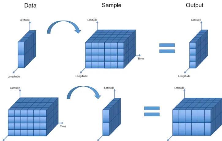
CIS can also collocate gridded data sets with differing di-mensionality. Where the sample array has dimensions that do not exist in the data, those dimensions are ignored for the purposes of the collocation and will not be present in the out-put. Where the data have dimensions that do not exist in the sample array, those dimensions are ignored for the purposes of the collocation and will be present in the output. There-fore, the output dimensionality is always the same as that of the input data, as shown in Fig. 4.

4.3.2 Ungridded to ungridded

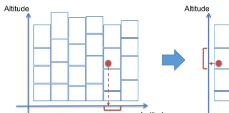
CIS is also able to collocate ungridded data. For ungridded to ungridded collocation the user is able to define a box to con-strain the data points which should be included for each sam-ple point. The schematic in Fig. 5 shows this box and its re-lation to the sample and data points. This box can be defined as a distance from the sample point in any of time, pressure, altitude or horizontal (haversine or great-circle) distance. In general, there may be many data points selected in this box. The user also has control over the kernel to be applied to

these data values. The default kernel, if none is specified, is the “moments” kernel, which returns the number of points selected, their mean value and the standard deviation on that mean as separate NetCDF variables in the output. Otherwise, the user can select only the mean or the nearest point in either time, altitude, pressure or horizontal distance. In this way, the user is able to find, for example, the nearest point in altitude within a set horizontal separation cut-off.

The specific process is outlined in Algorithm 3. For sim-plicity, we have assumed the dimensionality of the data sets is the same; in reality this need not be the case. CIS will collocate two data sets as long as both have the coordinates necessary to perform the constraint and kernel operations. Note also that this algorithm only outlines the basic princi-ples of the operations of the code; a number of optimizations are used in the code itself.

(9)

point-by-D. Watson-Parris et al.: Community Intercomparison Suite (CIS) 3101

Figure 4.This schematic shows the collocation of gridded data onto a gridded sampling with differing dimensionality. The output dimen-sionality is always the same as that of the input data.

Figure 5.This schematic shows the components involved in the col-location of ungridded data onto an ungridded sampling. The user-defined box around each sampling point provides a selection of data points which are passed to the kernel. Note that the resampled data points lie exactly on top of the sample points (which are not visible).

point comparison (which is shown in Algorithm 3, for sim-plicity).

4.3.3 Ungridded to gridded

For ungridded data points which are mapped onto a gridded sample, there are two options available. Either the ungridded data points can be binned into the bounds defined by each cell of the sample grid using the bin option, or the points can be constrained to an arbitrary area centred on the grid-ded sample point using the box option as described above. Either way, the moments kernel is used by default to return the number of points in each bin or box, the mean of their values and the standard deviation in the mean.

Stocker, T. F., Qin, D., Plattner, G. K., Tignor, M., Allen, S. K., Boschung, J., Nauels, A., Xia, Y., Bex, V., and Midgley, P. M. (Eds.): Climate Change 2013: The Physical Science Basis. Con-tribution of Working Group I to the Fifth Assessment Report of the Intergovernmental Panel on Climate Change, Cambridge

5

At-10

mos. Sci., 68, 2655–2670, 2011.

15

doi:10.5281/zenodo.59939, 2016.TS12

o.

INITIALIZEo_{= ∅} forj=1,...,Jdo

Algorithm 2Subsetting a gridded dataset G. Here we de-fine the algorithm for a two-dimensional dataset, although it can trivially be extended to higher dimensions. Given lower

ifcells have upper and lower boundsxuandxlrespectivelythen O= {Gij∀i, j:(ax≤xu_i ∨x_il≤bx)∨(ay≤y_ju∨y_jl ≤by)} else

onto a sampling set of coordinatessk ofK points. By

def-inition the output ois defined on the same spatio-temporal

sampling ass. The distance metricsDare defined for each

end for

Please

note

the

remarks

at

the

end

of

the

m

anuscript.

Algorithm 4 describes this process in more detail. As with Algorithm 3, we show here the operations performed, but not the exact code-path. In reality, a number of optimizations are made to ensure efficient calculations.

4.3.4 Gridded to ungridded

When mapping gridded data onto ungridded sample points, the options available are for the nearest neighbour value or a linearly interpolated value.

(10)

multi-3102 D. Watson-Parris et al.: Community Intercomparison Suite (CIS)

Figure 6.This schematic shows the collocation of gridded data onto an ungridded sampling where the altitude component of the data is defined on a hybrid height grid. CIS will first collocate the data in the coordinate dimensions (latitude, longitude, etc.) to extract a single-altitude column and then perform a second interpolation on the altitude coordinate.

Algorithm 4The ‘bin’ collocation of an ungridded dataset

onto a gridded sample set ofMmulti-dimensional cells, as

defined by the input file. Upper and lower bounds for each of

the cells of the dataset (bandarespectively) are

automati-cally deduced if not present in the data.

INITIALIZEO= ∅ form=1,...,Mdo

Q= {uj∀j:am<=rj<bm} Om=K(Q)

end for

www.geosci-model-dev.net/9/1/2016/ Geosci. Model Dev., 9, 1–19, 2016

ple variables with the same spatio-temporal coordinates only takes roughly as long as one variable.

4.4 Plotting

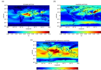
CIS also includes a comprehensive set of plotting capabili-ties, allowing the analysis and comparison of the whole vari-ety of data which can be read. This includes plots of aircraft flight tracks (see, e.g. Fig. 7) and satellite imagers (Fig. 8). It also allows the plotting of heat maps for gridded data as shown in the annual averages of aerosol optical thickness (AOT) plotted in Fig. 10. It also allows more detailed analy-sis of combined data sets, for example, by plotting collocated variables against each other as a scatter plot, and even as a 2-D histogram, for highlighting the distributions when there are many thousands of points, such as in Fig. 9.

The plotting output is highly customizable, with more than 35 different options available for specifying everything from the axes labels, to the colour of the coastlines. The user is also able to output the plots directly to screen for interactive visualization, including zooming and panning, or straight to image file (including .png, .jpg, .eps or .pdf) for publication-ready plots. A full description of the plotting syntax and available options is provided in the user man-ual (http://cis.readthedocs.org/en/stable/plotting.html)

Figure 7.An example scatter plot from a particular aircraft

mea-surement of ambient temperature as a function of latitude (xaxis)

and altitude (yaxis) produced directly by CIS. Note the

representa-tion of temperature as the colour of the scatter points.

along with an extended gallery of example plots (http://cis.readthedocs.io/en/stable/gallery.html).

4.5 Analysis

In addition to standard analysis options as described above, CIS allows general arithmetic operations to be performed be-tween different variables using the “eval” command. The two variables must be on the same spatio-temporal sampling, CIS will check that the data have the same dimensions but not that the points correspond to the same sampling. There are limit-less possibilities, but it enables, for example, the calculation of the difference between two collocated variables as demon-strated in Fig. 10. It also allows users to easily create a mask for a data set, for example, masking all of the mean output values from a collocation for which fewer than five points were used.

The basic structure of the eval command is as follows:

$ cis eval <datagroup>... <expr> <units>

where datagroup has already been described above (but variables can optionally take an alias to simplify the expres-sion), “expr” is the expression to evaluate and “units” is a string describing the units which should be assigned to the new variable (and must be CF compliant). Note that it is ac-tually possible to evaluate any Python expression with this command, including using the NumPy library, but that for security (in case CIS is being run as a different user or with elevated permissions for some reason) many built-in modules are unavailable.

(11)

Figure 8.An example plot showing the cloud liquid path over the Indian Ocean just off Malaysia, retrieved by the ESA Cloud CCI product MODIS Aqua (Hollmann et al., 2013).

exponent (α) for AOT (τλ) as measured by AERONET (AErosol RObotic NETwork) (http://aeronet.gsfc.nasa.gov/) at 870 and 440 nm, whereαis given by

α= − logτλ₁

τλ₂ logλ1 λ2

. (2)

This can be straightforwardly calculated using the follow-ing CIS command:

$ cis eval AOT_440,AOT_870: agoufou.lev20

"(-1)*(numpy.log(AOT_870/AOT_440)/ numpy.log(870./440.))" 1 -o alpha

Note that we have used the NumPy library to calculate the log of each of the variable arrays and have used the (AOT) variable names in the file forτ. The resultingαis then out-put to a CF-compliant NetCDF4 file for further analysis or processing.

4.6 Statistics

Users are also able to perform a basic statistical analysis on two variables using the stats command. This command has a very basic structure:

$ cis stats <datagroup>...

More than one datagroup may be specified, but the total number of variables declared in all the datagroups must be two (otherwise CIS will return an error message: “Stats com-mand requires exactly two variables (n were given)”). Again, they must both be on the same spatio-temporal sampling (otherwise CIS will return an error message that “operands could not be broadcast together”).

For example, the user might wish to examine the correla-tion between a model data variable and actual measurements or (as in the Ångström exponent example above) the corre-lation between a calculated and measured variable. The stats command will calculate the following:

1. the number of data points used in the analysis,

2. the mean and standard deviation of each data set (sepa-rately),

3. the mean and standard deviation of the absolute differ-ence (v₂−v₁),

4. the mean and standard deviation of the relative differ-ence ((v₂−v₁)/v₁),

5. the linear Pearson correlation coefficient, 6. the Spearman rank correlation coefficient and

7. the coefficients of linear regression (i.e.v₂=av₁+b), rvalue and standard error of the estimate.

Many of these values are calculated using the SciPy li-brary (Jones et al., 2001). The values are displayed on screen and can optionally be saved to a NetCDF4 file.

4.7 CIS as a Python library

CIS was primarily designed as a command line tool, however it is also straightforward to use some of the power of CIS in other Python modules or scripts. In particular, CIS provides an interface for reading any of the data sets which CIS sup-ports (either built-in or through user-supplied plugins). The data are returned in a well-documented data structure which provides straightforward access to the raw data, the coordi-nates and all associated metadata.

Further, because the data structure returned by these rou-tines are built on NumPy arrays, it is trivial to build these into existing Python-based data analysis routines. There is also an option to return the data as a Pandas (http://pandas. pydata.org) data frame. Pandas is an open-source data anal-ysis package providing, amongst other things, in-depth and easy-to-use time series analysis.

Version 2.0 of CIS is planned to include full support for all of the main CIS commands through the Python interface. For an outline of our future plans for CIS, please see www. cistools.net/roadmap.

5 Example scientific workflow

(12)

Figure 9.An example of plotting two collocated variables against one another as a scatter plot and also as a 2-D histogram. This can be useful for inspecting dense scatter plots.

the sake of this example, we use ECHAM6-HAM2 (first de-scribed by Stier et al., 2005), but as no scientific interpreta-tion of the comparison will be sought or offered, the details of the setup are not important.

As a first step it is often useful to inspect the contents of a data file to determine which variables it contains. This is straightforward using the “info” command:

$ cis info 920801_091128_Agoufou.lev20

This will return a list of the variables in the file, exactly as they should be passed to other commands. Variables can also be specified in the usual way to get more detailed information about any specific variables. Next, we might plot each of the data sets in order to examine their spatio-temporal extents and get a feel for the magnitudes of the AOT. We can plot the AERONET data with the following command:

$ cis plot AOT_675:

920801_091128_Agoufou.lev20

An example output plot is shown in Fig. 11. Note that the model data can not yet be plotted using CIS, as it is extended in latitude, longitude and time (if we tried, CIS would return an error message telling us “Data is not 1D or 2D – can’t plot it on a map.”). It could however be subsetted or aggregated to reduce the dimensionality before plotting.

Next, we might decide to subset the AERONET data to cover the same temporal range as the model data (which is for 2007):

$ cis subset AOT_675:

920801_091128_Agoufou.lev20 -t=[2007]

In order to quantitatively compare the values, we need to bring the model data onto the AERONET spatio-temporal sampling; this is straightforward using the collocation com-mand:

$ cis col TAU_2D_670nm: ECHAMHAM_AOT550_670.nc 920801_091128_Agoufou.lev20 -o echam_on_agoufou.nc

Note that this will linearly interpolate model data values in both space and time by default, though we could have chosen to use a nearest neighbour algorithm instead. Once we have two collocated data sets, we can calculate the point-wise dif-ference between the observations and the collocated model data using

$ cis eval TAU_2D_670nm: echam_on_agoufou.nc AOT_675: 920801_091128_Agoufou.lev20 "TAU_2D_670nm - AOT_675"

-o echam_aeronet_agoufou_diff.nc

We can also use the built-in analysis routines to give us an overview of the correlations between the two data sets using

thestatscommand:

$ cis stats TAU_2D_670nm: echam_on_agoufou.nc AOT_675: 920801_091128_Agoufou.lev20

This will print out to screen the mean and standard devia-tion in each data set, the absolute and relative differences be-tween them and the linear Pearson and Spearman rank corre-lation coefficients, as described in Sect. 4.6. Finally, in order to ensure a robust statistical comparison, we can then aggre-gate the collocated data in time to provide a yearly average:

$ cis aggregate TAU_2D_670nm: echam_aeronet_agoufou_diff.nc t -o echam_on_agoufou_diff_2007.nc

(13)

Figure 10.A comparison of annual average AOT at 550 nm between ECHAM and HadGEM3 across the globe.

multiple AERONET stations to produce a plot of the annual difference across the globe. Assuming we have performed the collocation and differencing over all of the stations, the aggregation step above is only slightly changed:

$ cis aggregate TAU_2D_670nm: echam_all_aeronet_diff.nc

t,x=[-180,180,0.5],y=[-90,90,0.5] -o echam_on_aeronet_diff_2007.nc

We have had to define a sufficiently fine spatial grid to maintain the spatial component of the difference. It is antic-ipated that future versions of CIS will support aggregation of ungridded data sets over only time, to support exactly this kind of workflow without the need to define an arbitrary grid (see http://cistools.net/roadmap for more details). Neverthe-less we can now plot this difference using a scatter plot as shown in Fig. 12 using the following command:

$ cis plot TAU_2D_670nm: echam_on_aeronet_diff_2007.nc --type scatter --nasabluemarble --cmap "RdBu_r"

Note that all of the cells in the aggregation with no points (where there are no AERONET stations) are masked in the output and thus not shown in the scatter plot.

Figure 11.CIS plot with default options for AOT observed from a single AERONET station.

6 Conclusions and summary

(14)

un-Figure 12.The difference between the annual average AOT mea-sured at AERONET stations around the world and ECHAM6-HAM2 modelled values. This plot only demonstrates a type of anal-ysis which is easy to perform with CIS; no scientific critique of these differences is offered.

gridded data sets, multiple gridded data sets or any combina-tion thereof.

Here, we have demonstrated the power and use of CIS – a new universal tool for the inter-comparison of model, remote sensing and in situ climate data. The open and extensible na-ture of the tool allows for the easy and reproducible colloca-tion, aggregacolloca-tion, subsetting and analysis of a huge variety of data sources on everything from laptops to large processing clusters. Further, the ability to extend the data sources com-patible with CIS through user-developed plugins provides the opportunity for a shared tool to serve a diverse community.

Further development of CIS is ongoing and we hope to include a number of new features in the future, such as an extended Python interface, hybrid gridded/ungridded data

structures and improved time series analysis, as outlined in our roadmap (www.cistools.net/roadmap). However,the growth of a user community (centred around our website) will help decide on the priority and best implementation of such features through user feedback and users actively en-gaging in development. All descriptions of functionality are correct as of version 1.4.0 (Watson-Parris et al., 2016), fu-ture releases and announcements can be found on the CIS website: http://cistools.net.

7 Code availability

The CIS source code is available on GitHub at https://github. com/cedadev/cis, and the binary is available for easy instal-lation on Windows, OS X and Linux through conda using the “conda-forge” or “cistools” channel (see http://cistools. net/get-started#installation for more details). CIS is also pre-installed on the UK JASMIN analysis platform (JASMIN runs a number of Red Hat Enterprise Linux 6 scientific com-puting virtual machines for which CIS is pre-installed. See http://www.jasmin.ac.uk for more details). Getting started documentation and the community plugin library is available at http://www.cistools.net. Detailed documentation and help pages can be found at http://cis.readthedocs.org.

(15)

Appendix A: Table of definitions

Table A1.A table of terms in this paper.

Term Definition

Aggregate the process of taking ungridded data and performing averaging over time and/or space

to produce a gridded output

Collocate the process of bringing two data sets on to the same spatial and temporal coordinates

Point-wise operation an operation carried out on each data point individually, usually on ungridded data

Gridded any regularly gridded data set for which points can be indexed using(i, j, k, . . .)where

i,jandkare integers

Ungridded any data which are not regularly gridded, in general it is assumed each(x, y, z)point is

(16)

Appendix B: Plugin development

In this section, we describe two specific ways that users are able to easily extend the functionality provided by CIS. The plugins are short pieces of Python code that users can write themselves and which CIS will then automatically incorpo-rate. Our website offers functionality for users to upload new plugins to be shared with the wider CIS community. Sub-mitted plugins will not be automatically included in the base CIS install, but can easily be downloaded and included by other users. If certain plugins prove popular then they will be tested, documented and included in the base install.

A detailed description of the development of CIS plug-ins and a number of increasingly in-depth tutorials can be found in the CIS documentation (http://cis.readthedocs.org/ en/stable/plugin_development.html); here, we provide only an overview of the basic plugin structures.

B1 Data plugins

CIS uses the notion of a “data product” to encapsulate the in-formation about different types of data. Users can write their own products for reading in different types of data, referred to as plugins. These products (or plugins, if provided by the user) are concerned with interpreting the raw data and their coordinates and producing a single self-describing data ob-ject conforming to the CommonData interface (see Fig. 1). They follow a defined structure so that they can be automati-cally included and used by the tool. We briefly describe that structure here.

All plugins must subclass the AProductabstract class

(this class defines the structure described here and indicates to CIS the type of plugin the user has supplied), and are there-fore forced to provide an implementation for the following methods:

– get_file_signature(self) returns a list of

regular expressions to match the product’s file-naming convention. CIS will use this to decide which data prod-uct to use for a given file. The first prodprod-uct with a sig-nature that matches the filename will be used.

– create_coords(self, filenames)is used to

return the coordinates from one or more files. Note that this method may have to make certain assumptions about the file in order to return a single coordinate set.

– create_data_object(self, filenames,

variable)creates and returns a CommonData object

for a given variable from a list of filenames.

The underlying I/O layers are also available for the plugins to use (such as NetCDF reading) which ensures the writing of plugins is as straightforward as possible.

B2 Collocation

Users can also write their own plugins for performing the col-location of two data sets. There are three main objects used in the collocation which the user is free to override: the col-locator, the constraint and the kernel. The basic design is that the collocator loops over each of the sample points, calls the relevant constraint to reduce the number of data points and then calls the kernel which returns a single value for the col-locator to store.

The main plugin which is available is the collocation method itself. A new one can be created by subclassing

Collocator and providing an implementation for the

main “collocate” method. This method takes a number of points and applies the given constraint and kernel methods on the data for each of those points. It is responsible for re-turning the new data object to be written to the output file.

The constraint object limits the data points for a given sample point in some way. The user can also add a new con-straint method by subclassingConstraintand providing

an implementation for the methodconstrain_points.

The final plugin type is theKernelwhich is used to

con-vert the constrained points into values in the output, many examples of which are listed in Table 4.

(17)

The Supplement related to this article is available online at doi:10.5194/gmd-9-3093-2016-supplement.

Acknowledgements. We would like to acknowledge the guidance

and support of Stephen Pascoe through his role in CEDA during the first phases of development, and Caroline Poulsen (Remote Sensing Group, EOAS Division, RAL Space) who provided invaluable user feedback. The first phase of development was supported by e-infrastructure capital grants for JASMIN from the Science and Technology Facilities Council (ST/K000594/1). Subsequent development was supported by Natural Environment Research Council capital funding for JASMIN. Scientific support has been provided by the Global Aerosol Synthesis and Science Project (GASSP), Natural Environment Research Council (NE/J022624/1). The research leading to these results has received funding from the European Research Council under the European Union’s Seventh Framework Programme (FP7/2007–2013)/ERC grant agreement no. FP7-280025. We thank the AERONET principal investigators (PIs) and their staff for establishing and maintaining the AERONET sites used in the examples here. We are also grateful to the ESA Cloud CCI project and to NASA for the underlying MODIS data sets which went into one of the examples used.

Edited by: F. O’Connor

Reviewed by: two anonymous referees

References

Beck, K.: Extreme Programming Explained: Embrace Change, An Alan R. Apt Book Series, Addison-Wesley, Boston, Mas-sachusetts, 2000.

Beck, K.: Test-Driven Development by Example, Addison-Wesley, Boston, Massachusetts, 2003.

Bentley, J. L.: Multidimensional Binary Search Trees Used for As-sociative Searching, Commun. ACM, 18, 509–517, 1975. Boucher, O., Randall, D., Artaxo, P., Bretherton, C., Feingold, G.,

Forster, P., Kerminen, V. M., Kondo, Y., Liao, H., Lohmann, U., Rasch, P., Satheesh, S. K., Sherwood, S., Stevens, B., and Zhang, X. Y.: Clouds and Aerosols, in: Climate Change 2013: The Phys-ical Science Basis. Contribution of Working Group I to the Fifth Assessment Report of the Intergovernmental Panel on Climate Change, edited by: Stocker, T. F., Qin, D., Plattner, G. K., Tig-nor, M., Allen, S. K., Boschung, J., Nauels, A., Xia, Y., Bex, V., and Midgley, P. M., pp. 571–658, Cambridge University Press, Cambridge, United Kingdom and New York, NY, USA, 2013. Eyring, V., Bony, S., Meehl, G. A., Senior, C. A., Stevens, B.,

Stouffer, R. J., and Taylor, K. E.: Overview of the Coupled Model Intercomparison Project Phase 6 (CMIP6) experimen-tal design and organization, Geosci. Model Dev., 9, 1937–1958, doi:10.5194/gmd-9-1937-2016, 2016a.

Eyring, V., Righi, M., Lauer, A., Evaldsson, M., Wenzel, S., Jones, C., Anav, A., Andrews, O., Cionni, I., Davin, E. L., Deser, C., Ehbrecht, C., Friedlingstein, P., Gleckler, P., Gottschaldt, K.-D., Hagemann, S., Juckes, M., Kindermann, S., Krasting, J., Kunert, D., Levine, R., Loew, A., Mäkelä, J., Martin, G., Mason, E.,

Phillips, A. S., Read, S., Rio, C., Roehrig, R., Senftleben, D., Sterl, A., van Ulft, L. H., Walton, J., Wang, S., and Williams, K. D.: ESMValTool (v1.0) – a community diagnostic and perfor-mance metrics tool for routine evaluation of Earth system models in CMIP, Geosci. Model Dev., 9, 1747–1802, doi:10.5194/gmd-9-1747-2016, 2016b.

Gleckler, P., Doutriaux, C., Durack, P., Taylor, K., Zhang, Y., Williams, D., Mason, E., and Servonnat, J.: A More Pow-erful Reality Test for Climate Models – Eos, Eos, 97, doi:10.1029/2016EO051663, 2016.

Hewitt, H. T., Copsey, D., Culverwell, I. D., Harris, C. M., Hill, R. S. R., Keen, A. B., McLaren, A. J., and Hunke, E. C.: Design and implementation of the infrastructure of HadGEM3: the next-generation Met Office climate modelling system, Geosci. Model Dev., 4, 223–253, doi:10.5194/gmd-4-223-2011, 2011.

Hollmann, R., Merchant, C. J., Saunders, R., Downy, C., Buch-witz, M., Cazenave, A., Chuvieco, E., Defourny, P., de Leeuw, G., Forsberg, R., Holzer-Popp, T., Paul, F., Sandven, S., Sathyen-dranath, S., van Roozendael, M., and Wagner, W.: The ESA mate Change Initiative: Satellite Data Records for Essential Cli-mate Variables, B. Am. Meteorol. Soc., 94, 1541–1552, 2013. Jones, E., Oliphant, T., Peterson, P., et al.: SciPy: Open source

sci-entific tools for Python, available at: http://www.scipy.org/ (last access: 1 August 2016), 2001.

Kipling, Z., Stier, P., Schwarz, J. P., Perring, A. E., Spackman, J. R., Mann, G. W., Johnson, C. E., and Telford, P. J.: Constraints on aerosol processes in climate models from vertically-resolved aircraft observations of black carbon, Atmos. Chem. Phys., 13, 5969–5986, doi:10.5194/acp-13-5969-2013, 2013.

Langerock, B., De Mazière, M., Hendrick, F., Vigouroux, C., Desmet, F., Dils, B., and Niemeijer, S.: Description of algo-rithms for co-locating and comparing gridded model data with remote-sensing observations, Geosci. Model Dev., 8, 911–921, doi:10.5194/gmd-8-911-2015, 2015.

Lawrence, B. N., Bennett, V. L., Churchill, J., Juckes, M., Ker-shaw, P., Oliver, P., Pritchard, M., and Stephens, A.: The JASMIN super-data-cluster, arXiv:1204.3553 [cs.DC], 2012.

Levy, R. C., Leptoukh, G. G., Kahn, R., Zubko, V., Gopalan, A., and Remer, L. A.: A Critical Look at Deriving Monthly Aerosol Op-tical Depth From Satellite Data, IEEE T. Geosci. Remote Sens., 47, 2942–2956, 2009.

Maneewongvatana, S. and Mount, D. M.: It’s Okay to Be Skinny, If Your Friends Are Fat, in: Center for Geometric Computing 4th Annual Workshop on Computational Geometry, 1999.

Met Office: Iris: A Python library for analysing and vi-sualising meteorological and oceanographic data sets, doi:10.5281/zenodo.51860, 2016.

Schutgens, N. A. J., Gryspeerdt, E., Weigum, N., Tsyro, S., Goto, D., Schulz, M., and Stier, P.: Will a perfect model agree with per-fect observations? The impact of spatial sampling, Atmos. Chem. Phys., 16, 6335–6353, doi:10.5194/acp-16-6335-2016, 2016a. Schutgens, N. A. J., Partridge, D. G., and Stier, P.: The

impor-tance of temporal collocation for the evaluation of aerosol mod-els with observations, Atmos. Chem. Phys., 16, 1065–1079, doi:10.5194/acp-16-1065-2016, 2016b.

(18)

Stier, P., Feichter, J., Kinne, S., Kloster, S., Vignati, E., Wilson, J., Ganzeveld, L., Tegen, I., Werner, M., Balkanski, Y., Schulz, M., Boucher, O., Minikin, A., and Petzold, A.: The aerosol-climate model ECHAM5-HAM, Atmos. Chem. Phys., 5, 1125–1156, doi:10.5194/acp-5-1125-2005, 2005.

Stocker, T. F., Qin, D., Plattner, G. K., Tignor, M., Allen, S. K., Boschung, J., Nauels, A., Xia, Y., Bex, V., and Midgley, P. M. (Eds.): Climate Change 2013: The Physical Science Basis. Con-tribution of Working Group I to the Fifth Assessment Report of the Intergovernmental Panel on Climate Change, Cambridge University Press, Cambridge, United Kingdom and New York, NY, USA, 2013.

Suzuki, K., Stephens, G. L., van den Heever, S. C., and Nakajima, T. Y.: Diagnosis of the Warm Rain Process in Cloud-Resolving Models Using Joint CloudSat and MODIS Observations, J. At-mos. Sci., 68, 2655–2670, 2011.

Teixeira, J., Waliser, D., Ferraro, R., Gleckler, P., Lee, T., and Potter, G.: Satellite Observations for CMIP5: The Gen-esis of Obs4MIPs, B. Am. Meteorol. Soc., 95, 1329–1334, doi:10.1175/BAMS-D-12-00204.1, 2014.

Watson-Parris, D., Schutgens, N. A. J., Cook, N., Kipling, Z., Ker-shaw, P., Gryspeerdt, E., Stier, P., and Lawrence, B.: CIS: v1.4.0, doi:10.5281/zenodo.59939, 2016.