AN SUPPORT VECTOR REGRESSION BASED
NONLINEAR MODELING METHOD FOR SIC MESFET
Y. Xu, Y. Guo, R. Xu, L. Xia, and Y. Wu
School of Electrical Engineering
University of Electronic Science and Technology of China (UESTC) Chengdu, China
Abstract—An approach for the microwave nonlinear device modeling technique based on a combination of the conventional equivalent circuit model and support vector machine (SVM) regression is presented in this paper. The intrinsic nonlinear circuit elements are represented by Taylor series expansions, coefficients of which are predicted by its support vector regression (SVR) model. Example of a SiC MESFET nonlinear model is demonstrated, and good results is achieved.
1. INTRODUCTION
SiC MESFETs are popular devices for power amplifier design in high-power and high-temperature applications because of SiC’s superior properties, such as high breakdown voltage, high thermal conductivity, and high saturated electron velocity [1]. The development of SiC devices in wireless applications provides the impetus of researching in the area of nonlinear modeling, which is useful for device performance analysis in designing microwave circuits and characterizing the device technological process.
configurations, and on-convex quadric minimization may result in multiple minima [4].
A new microwave active device nonlinear modeling technique based on the combination of the conventional closed-form equation models and support vector machine (SVM) is proposed. Different from ANN, the SVM is based on structural risk minimization (SRM) principle and resolving convex quadratic program (QP), which shows more powerful generalization ability than ANN [5, 6]. In this paper, example of SiC MESFET nonlinear modeling utilizing the proposed support vector regression (SVR) based modeling technique are demonstrated. The main frequency independent intrinsic nonlinear elements (source-drain current Ids, nonlinear capacitances Cgs and
Cgd) are, firstly, modeled by SVR. By using Taylor series expansion of intrinsic nonlinear elements, their coefficients are predicted by related SVR models. With this method, the nonlinear characteristic of SiC MESFET can than be good described in numerical way while preserving the original physical meaning of closed-form equation models.
The organization of this paper is as follows: Section 2 summarizes the theory of support vector regression. Section 3 describes the structure of SiC MESFET used in this paper and the proposed SVR-based nonlinear modeling technique. Section 4 shows the results by using proposed method applied to SiC MESFET.
2. SUPPORT VECTOR REGRESSION
SVMs are state-of-the-art tools for linear and nonlinear input-output knowledge discovery [7, 8]. Given a training dataset (yi, xi), i = 1, 2, . . . , n, xi ∈ Rm, n is the size of training data. SVR tries to find the mapping functionf(x) between the input variable and the desired output variable. Traditional regression method find the regression functionf(x) by the rule of empirical risk minimization principle, i.e., minimize:
Remp[f] = 1
n
n
i=1
L(f(xi)−yi) (1)
with L(x, y, f) = |y−f|ε = max{0,|y−f| −ε}. L(f(xi) − yi) represents the error function, ε is the insensitive loss function. yi is real value, f(xi) is the prediction value.
principle, which minimize the following cost function:
1 2w
2+C·R
emp[f] (2) where 12w2 is the term characterizing the modeling complexity. C
is a regularization which determines the trade off between model complexity and empirical loss function. After some reformulations and introduction of the slack variables: ξi,ξ∗i. Equation (2) is transformed into primal problem:
minimize:
1 2w
2+C· 1
n
(ξi+ξ∗i) (3) subject to:
(w·xi) +b−yi≤ε+ξi
yi−(w·xi) +b≤ε+ξi∗
ξi>0, ξ∗i >0, ε >0.
According to [5], an improved SVR has been presented, Equation (3) can be changes to minimize:
minφ(w, b) = 1 2w
2+C
νε+ 1/l
l
i=1
Li
s.t. yi =< w, xi >+b≥1−Li, Li ≥0, ∀i (4) whereC (penalty parameter) is a regularization which determines the trade off between model complexity and empirical loss function, ε is tolerance of termination criterion, and v (0< v <1) is a constant.
Introducing Lagrange multipliers to solve this problem of convex optimization and making some substitutions, we arrive to the Wolfe dual of the optimization problem:
maximize:
W(α, α∗) =(αi−α∗i)yi− 1 2
n
i,j=1
subject to: n i=1
(α∗i −αi) = 0
αi ∈ 0,
C n
α∗i ∈ 0,C n
n
i=1
(α∗i −αi)≤C·ν
In order to expand the method to nonlinear decision functions, the input space projects to another higher-dimensional dot product space
F, called feature space, via a nonlinear map ϕ: Rm → Fd(d m). In this new space the optimal hyperplane is derived. Nevertheless, by using kernel functions which satisfy the Mercer’ theorem, it is possible to make all the necessary operations in the input space by using< ϕ(xi),ϕ(xj)>=K(xi,xj). The regression estimation function is formulated in terms of these kernels:
f(x) = l
i=1
(αi−α∗i)K(xi, x) +b (6) whereaianda∗i are Lagrange multiples,K(xi,x) is the kernel function.
K is a symmetric positive definite function, which satisfies Mercer’s condition.
It is easy to demonstrate that < ϕ(x), ϕ(y) > is given the derivative of withK(x,y) respect tox [9]. Accordingly, thenth-order derivatives off(x) is
g(n)(x) = l
i=1
(αi−α∗i)K(n)(xi, x) (7) This developed SVR model can then be used to predict outputs for given inputs that were not included in the training data, and then th-order derivatives of outputs.
3. NONLINEAR MODELING OF SIC MESFETS BASED ON SVR TECHNIQUES
An 1µm×300µm 4H-SiC MESFET is modeled in this paper. This device consists of a 0.15-µm cap layer (Nd = 5×1015cm−3),
(Nd = 1.5×1015cm−3) on a semi-insulated 4H-SiC substrate. The buffer layer can prevent damage and deep level impurities in the substrate from the active layer. Due to the lack of p-doping source at the moment, we use an unintentionally weak n-type layer as the buffer in order to minimize the influence of substrate. The caculated cut-off frequency (fT) and maximum frequency of oscillation (fmax)
are 6.7 GHz and 25 GHz, respctively.
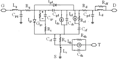
The basic topology of the empirical model for SiC MESFETs is shown in Fig. 1. The Angelov non-linear gate capacitances model (Cgs,Cgd) and a modified drain-source current (Ids) equation based on Angelov model is used, and detail information about empirical model are showed in [2]. The model has been implemented into ADS as a user-defined model, and its validity has been proved in predicting electrical performance of SiC MESFETs. The simulatedS-parameters of empirical model at different bias will construct the data needed for a SVR model. The simulation has been accomplished by ADS with directly 50 Ω input-output terms.
Figure 1. Equivalent circuit of the empirical model for SiC MESFETs.
Only there main intrinsic nonlinear element (Cgs, Cgd, and Ids) will be considered in our method for simple demonstration. Similar to ANN methods [3], each main intrinsic nonlinear element can be modeled by independent SVR models
Cgs = fSV R(Vds, Vgd) (8)
Cgd = fSV R(Vds, Vgd) (9)
model can be carried out by using the similar way of ANN methods [3]. However, the physical mechanism of nonlinear model is still not clearly enough. Here, a more physical nonlinear modeling method is proposed based on above SVR models.
Typically, the transistor is polarized in a bias point (Vds0, Vgs0),
and the incremental drain-to-source and gate-to source voltages, vds and vgs, are applied over this DC polarization. With these premises, it is necessary to accurately reproduce the nonlinear elements f(Vds,
Vgs) = F(Vds0, Vgs0, vds, vgs) dependence and its derivatives with
respect to the incremental voltages. In applications of amplifiers and mixers, the usual is to consider up to the third order intermodulation distortion (IMD) [11]. As a result, the nonlinear elementsQg(Vds, Vgd) can be expressed as Taylor series expansion
Qg(Vgs, Vgd) = Qg(Vgs0, Vgd0) +Cgs1vgs+Cgd1vgd+Cgs2vgs2 +Cgsgdvgsvgd+Cgd2v2gd+Cgs3v3gs+Cgs2gdv2gsvgd +Cgsgd2vgsvgd2 +Cgd3vgd3 (11) Accordingly, the Cgs(Vds, Vgs), Cgd(Vds, Vgs) and Ids(Vds, Vgs) expansions are as follows:
Ids(Vds, Vgs) = Ids(Vds0, Vgs0) +Gmvgs+Gdvds+Gm2vgs2 +Gmdvgsvds+Gd2vds2 +Gm3vgs2 +Gm2dvgs2 vds +Gmd2vgsvds2 +Gd3vds3 (12)
Cgs(Vgs, Vgd) = Cgs1+ 2Cgs2vgs+Cgsgdvgd+ 3Cgs3v2gs
+2Cgs2gdvgsvgd+Cgsgd2vgd2 (13)
Cgd(Vgs, Vgd) = Cgd1+ 2Cgd2vgd+Cgsgdvgs+ 3Cgd3v2gd
+2Cgsgd2vgsvgd+Cgs2gdvgs2 (14) whereQg(Vds0, Vgs0) andIds(Vds0, Vgs0) is the static DC values at bias
point, and (Gm, . . ., Gd3, Cgs1, . . ., Cgd3) are coefficients related to
thenth-order derivatives valuated at the bias point.
Different from previous work on Ids(Vds, Vgs) [2, 12], the coefficients of each nonlinear elements are directly predicted by SVR
nth-order derivatives models for each nonlinear elements. Benefit to the great generalization ability of SVM, the coefficients of nonlinear elements model can be accurately extracted. For example,
Gm =
∂IdsSV R(Vgs, Vds)
∂Vgs
Cgsgd =
∂CgsSV R(Vgs, Vgd)
∂Vgd
= ∂C SV R
gd (Vgs, Vgd)
∂Vgd
(16)
Cgd3 =
1 3
∂2CgdSV R(Vgs, Vgd)
∂V2
gd
(17)
Cgs1 = CgsSV R(0,0)
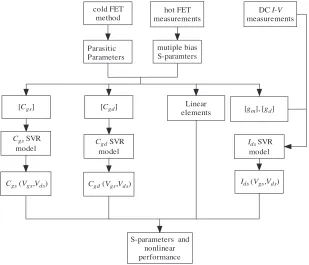
The detailed flow chat is showed in Fig. 2, where [Cgs], [Cgd], [gm] and [gd] represents the calculated discrete values at different bias.
Linear elements
[Cgs] [Cgd]
cold FET method
Parasitic Parameters
hot FET measurements
mutiple bias S-paramters
CgsSVR
model
CgdSVR model
DCI-V
measurements
IdsSVR
model
S-parameters and nonlinear performance
[gm], [gd]
Cgs(Vgs,Vds) Cgd(Vgs,Vds) Ids(Vgs,Vds)
Figure 2. The proposed SVR based nonlinear modeling flow chat.
The modeling technique can be carried out with the following procedures:
a) Measurement of the dc I-V and the multiple biased S-parameter for a microwave device.
b) Extraction of the parasitic parameters of microwave device using cold FET method.
d) Modeling of the intrinsic capacitances and dc current by using SVR technique.
e) Reconstruction of nonlinear elements expression by calculation of thenth-order derivatives of nonlinear elements SVR models. f) Calculation of the S-parameters and nonlinear performance by
using the nonlinear elements in the nonlinear circuit simulator.
4. MODEL VERIFICATION
LIBSVM-matlab code [14] is used as a basis to implement SVR model.
v-SVR based on radial basis function (RBF) kernel function has been considered in our regression experiments. The parameters (ε,v,Cand
γ) are extracted by trying with different variable value. The quality of each model is evaluated as its prediction accuracy, measured by mean squared error (M SE):
M SE = 1
N
N
i=1
(yi−xi)2 (18)
xi is the value of simulatedS-parameters of empirical model,yi is the SVR model predicted value andN is the number of validation data.
Table 1 showed the SVR variables and samples for training and test data. The same variables (bias points) are selected for each nonlinear element. And the total number of training data is 30 points, which means only 30 sets of S-parameters and DC I-V data are needed for build a nonlinear model with this method. And the samples are selected with the same steps, which mean the SVR model
Table 1. SVR variables and samples selection.
Data Training Data Testing Data Para. Min Max Step Min Max Step
Vds/V 0 20 4 0 20 1
Vgs/V −15 0 −3 −15 0 −1.5
Table 2. Results of SVR model.
Data Training Data Testing Data Para./Unit Ids/mA Cgs/pF Cgd/pF Ids/mA Cgs/pF Cgd/pF
0 5 10 15 20 0
10 20 30 40 50 60 70 80 90
Ids /mA
Vds/V
0 5 10 15 20
0.04 0.06 0.08 0.1 0.12 0.14 0.16 0.18 0.2
Vds/V Cgs
/PF
0 5 10 15 20
0.02 0.04 0.06 0.08 0.1 0.12 0.14 0.16 0.18
Cgd
/PF
Vds/V
(a) (b)
(c)
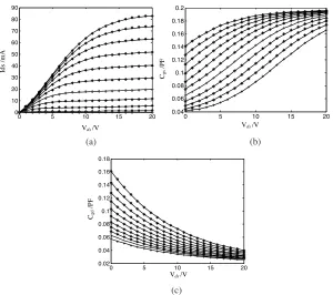
Figure 3. The plots of predicted results vs. testing samples. (a) Plot of predictedIds results (solid line) vs. testing samples (star), (b) Plot of predictedCgs results (solid line) vs. testing samples (star), (c) Plot of predictedCgd results (solid line) vs. testing samples.
is a robust model that with little dependence of the training samples distribution while the results of ANN models are greatly depend on sample selection. Table 2 shows the M SE results of training and testing data. And Fig. 3 is the plots of predicted results vs. testing samples for each nonlinear element. The results reveal that the SVR model can accurately predict each nonlinear element in less than 1 minute on an Intel Pentium IV 3.0 GHz with 1 GB of memory and running Windows XP. Besides, it is great convenient that the parameters (ε, v, C and γ) for each SVR model are the same. It means only four parameters are needed for the nonlinear model, while ANN based method usually require several hundred parameters [3].
-0.4 -0.3 -0.2 -0.1 0.0 0.1 0.2 0.3 0.4
-0.5 0.5
20GHz
500MHz
20GHz
500MHz
10S12
S21
S12
S11
(a)
S21
-0.6 -0.4 -0.2 0.0 0.2 0.4 0.6
-0.8 0.8
500MHz
20GHz
500MHz
S11
S12 20GHz
10S12
(b)
Figure 4. Comparison of S-parameters between the empirical model (circles) and the SVR based model (solid line) of SiC MESFET in the frequency range of 500 MHz–20 GHz. bias: (a)Vgs=−2 V,Vds = 20 V, (b)Vgs=−7 V, Vds = 20 V.
10
-10 20
-50
-150 50
f0
2f0
3f0
Pout
/dBm
Pin/dBm 0
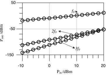
(Pout) are that the simulations were accomplished by directly 50 Ω input-output terms and the simulatios frequency is far over fT. The data are selected for demonstration purpose of the proposed method, and the good agreements show the validation of the proposed method.
5. CONCLUSION
An approach for the microwave nonlinear device modeling technique based on a combination of the conventional equivalent circuit model and support vector machine (SVM) regression is presented in this paper. The example of SiC MESFET modeling shows that the proposed method can provide fast and accurately modeling, whilst preserve the advantages of closed-form equation model. This technique is very useful for device performance analysis in designing microwave circuits and characterizing the device technological process for relatively new compound semiconductors such as GaN and SiC.
REFERENCES
1. Charles, E. W., “Comparison of SiC, GaAs, and Si RF MESFET power densities,” IEEE Transaction on Electron Device Letters, Vol. 16, 451–453, 1995.
2. Xu, Y., “Large-signal modeling of SiC MESFETs,” Master dissertation, University of Electronic Science and Technology of China, 2007.
3. Zhang, Q. J., K. C. Gupta, and V. K. Devabhaktuni, “Artificial neural networks for RF and microwave design — from theory to practice,”IEEE Transactions Microwave Theory and Techniques, Vol. 51, 1339–1350, 2003.
4. Xia, L., R. Xu, and B. Yan, “LTCC interconnect modeling by support vector regression,” Progress In Electromagnetics
Research, PIER 69, 67–75, 2007.
5. Bermani, E., A. Boni, A. Kerhet, and A. Massa, “Kernels evaluation of SVM based estimatiors for inverse scattering problems,”Progress In Electromagnetics Research, PIER 53, 167– 188, 2005.
6. Yang, Z. Q., T. Yang, Y. Liu, and S. H. Han, “MIM capacitor modeling by support vector regression,” Journal of
Electromagnetic Waves and Applications, Vol. 22, 61–67, 2008.
range using support vector machine regression,” Progress In
Electromagnetics Research, PIER 70, 247–256, 2007.
8. Xu, Y., “Modeling of SiC-MESFETs by using support vector machine regression,” Journal of Electromagnetic Waves and
Applications, Vol. 21, 1489–1498, 2007.
9. L´azaro, M., F. P´erez-Cruz, and A. Art´es-Rodr´ıguez, “Learning a function and its derivative forcing the support vector expansion,”
IEEE Signal Processing Letters, Vol. 12, 194–197, 2005.
10. Perez-Cruz, F., M. Lazaro, and A. Artes-Rodriguez, “Mutidimen-sonal SVM to include the samples of the derivatives in the recon-struction of a function,”2004 European Signal Processing Confer-ence, 597–600, Vienna, Sep. 2004.
11. Pedro, J. C. and J. P´erez, “Accurate simulation of GaAs MESFETs intermodulation using a new drain-source current model,” IEEE Transactions Microwave Theory and Techniques, Vol. 42, 25–33, 1994.
12. Santamar´ia, I., M. L´azaro, C. J. Pantale´on, J. A. Garc´ia, A. Taz´on, and A. Mediavilla, “A nonlinear MESFET model for intermodulation analysis using a generalized radial basis function network,”Neurocomputing, Vol. 25, 1–18, 1999.
13. Dambrine, G., A. Cappy, F. Heliodore, and E. Player, “A new method for determining the FET small-signal equivalent circuit,”
IEEE Transactions Microwave Theory and Techniques, Vol. 36,
1151–1159, 1988.
14. Chang, C. C. and C. J. Lin, LIBSVM 2.81(2006): A library for support vector machines. Available: http://www.csie.ntu.edu. tw/∼cjlin/libsvm.
15. Wang, L., R. M. Xu, Y. C. Guo, and B. Yan, “A temperature-dependent current model for phemt on GaAs,” Journal of
Electromagnetic Waves and Applications, Vol. 22, 39–46, 2008.
16. Shi, Z. G., “Microwave chaostic colpitts oscillator: Design, implementation and application,” Journal of Electromagnetic