Michael Beye1and Thijs Veugen1,2
1
Information Security and Privacy Lab, Faculty of Electrical Engineering, Mathematics and Computer Science, Delft University of Technology, The Netherlands
2
Security Group, TNO, The Netherlands [email protected]
Abstract. Randomized hash-lock protocols for Radio Frequency IDen-tification (RFID) tags offer forward untraceability, but incur heavy search on the server. Key trees have been proposed as a way to reduce search times, but because partial keys in such trees are shared, key com-promise affects several tags. Butty´an et al. have quantified the resulting loss of anonymity in the system, and proposed specific tree properties in an attempt to minimize this loss. We will further improve upon these results, and provide a proof of optimality. Finally, our proposals are com-pared to existing results by means of simulation.
Key words: RFID, Hash-lock protocol, key-tree, anonymity, anonymity set
1 Introduction
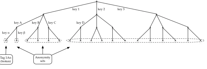
We consider the problem of authenticating many Radio Frequency IDentifica-tion (RFID) tags through randomized hash-lock protocols, in an efficient way. The tags are authenticated towards the reader through a challenge-response mechanism. Each tag authenticates itself using some secret key combined with a random value (nonce). To authenticate the tag, the reader will have to check the keys of all tags combined with all possible random values, in order to find a match. Since this task is very intensive for the reader, a key-tree is used. Each leaf of the tree represents a tag, and each edge corresponds to a specific key. Every tag is assigned the keys that lie on its path from the root of the tree (see Fig. 1). During the authentication protocol, a tag is authenticated step by step, i.e. edge by edge, such that the computational load of the reader, and thus the total authentication time, is lowered.
However, the authentication mechanism should still remain secure. If hardware-level tampering is taken into account, keys that were assigned to compromised tags can become known to the adversary. Because partial keys are shared between neighboring tags in the tree, several additional tags may be partially broken as
⋆
well. How to construct the tree such that the number of (partially) broken tags will be minimal in case of one or more compromises?
This paper considers the trade-off between efficiency (minimizing authenti-cation time), and security (minimizing the impact of tag compromise on neigh-boring tags), of such authentication mechanisms.
The layout of this paper is as follows: Section 2 will outline related work, with an emphasis on Butty´an et al.’s previous work on the optimization of key-trees. In Section 3, Butty´an’s optimization problem is rephrased, an improved solution is suggested, and its effect is quantified. Finally, conclusions will be drawn in Section 4.
2 Related Work
Hash-chain protocols are meant to provide forward untraceability, by updating
tag IDs in a one-way manner. This way, past IDs cannot be recovered, even through tampering. Examples are OSK (by Ohkubo, Suzuki and Kinoshita in [14]) and Yeo’s protocol [16]. In [1], Avoine et al. suggest applying time-memory trade-offs (based on Hellmann tables [9]) to hash-chain protocols (namely OSK and an improved version thereof). In [2] they extend this trade-off with so-called rainbow tables and checkpoints to further improve efficiency. Hash-chain protocols have weaknesses, including protocol exhaustion (when the end of a chain is reached, tags can no longer update their IDs and become traceable) and
desynchronization (server and tag chains can become out of synch if tags are
queried by third parties).
A different class of hash-based authentication schemes calledHash-lock
pro-tocols (due to Weis et al.) was devised to solve the aforementioned problems.
Tags are locked and unlocked, using hashes of their ID as the key. The static
hash-lock scheme [15] is vulnerable to both replay attacks and tracking, but in
the same paper, Weis et al. offer therandomized hash-lock scheme as a solution to such attacks: it adds tag freshness (a nonce generated by the tag) to pre-vent reader impersonation and tracking. The nonce is used as a challenge, and is hashed together with the tag’s ID to form a one-time-use authentication key (the expected response). Juels and Weis [10] later added reader freshness to also prevent tag impersonation.
Note that precomputation cannot be used in these protocols, because the use of freshness makes the search space too large – one would need to compute values not only for each tag, but for each tag ID in combination with all possible nonces. Other solutions are required to reduce search complexity.
Molnar was the first to propose using atree of secrets for RFID tags [11]. Although originally used for a system built around exclusive-OR and a pseudo-random function, it can be applied to other challenge-response building blocks. Damg˚ard and Østergaard Pedersen [5] use the same concept, but speak of
cor-related keys. Nohara et al. in their “K-steps protocol” ([12], also dubbed NIBY)
rather than correlated keys, and their trees are unconventional (being of non-uniform depth). Note that all these approaches use a sequence of group- and sub-group IDs to quickly and gradually narrow down a tag’s identity. As Molnar mentions, partial keys in such a tree should be chosen independently and
uni-formly from a key space of sufficient entropy. Failure to do so would make the
system vulnerable to attack. If partial keys are chosen properly, the adversary will have a large key space to search, while the owner of the system can efficiently search through a limited subspace (the actual tree).
The trade-off that exists between efficiency and security in tree-based pro-tocols was already pointed out by Avoine [1], with respect to Molnar’s original trees. Because tags share their partial keys, if one tag is compromised (i.e. has its memory probed through invasive tampering), an adversary learns partial keys for several other tags as well. This will enable him to decipher their responses in some of the verification steps, resulting in reduced anonymity and facilitating tracking. Nohl and Evans [13] try to quantify this more precisely. They distin-guish between scenarios where compromised tags are chosen in a selective or a
random way, and compute theinformation leakage measured in bits.
A paper of particular interest is by Butty´an et al. [4], where the concept of trees withvariable branching factors is introduced, to better preserve anonymity in case of attack. Our work provides an optimization of Butty´an’s solution.
In [8] Butty´an tries to further improve the balance between complexity and privacy in a new “group-based” authentication protocol. In short, the tags are divided intoλgroups, where each group shares a group-key. Every tag also has an ID. This group-based scheme can be seen as a tree of depth 2, where every group-ID is tried, but the last stage (unique ID) only requires one decryption instead of exhaustive search. This means that the tree can be even wider at the top than a Butty´an tree, and thus attains a higher anonymity score. However, we choose not to follow this example because we believe that the group-based authentication protocol in [8] has inherent flaws, as will be explained in Section 4.
2.1 Notation
This paper bases its notation on that of Butty´an in [4], but makes minor exten-sions:
– T ={t1,· · ·, tN}: set of all tags in the system – N: size ofT, or actual number of tags in the system – N′: number of leaves in the tree (Q
(B)), or maximum number of tags in the system,N′ ≥N
– c: number of compromised tags
– P(ti): helper function that returns the anonymity set to which tagti belongs – Pj: anonymity setj, 0≤j≤ℓ
– ℓ: number of anonymity sets in a given configuration – S: size of a given anonymity set
– ¯Sh−i(c): expected values of ¯S (averaged over all configurations containing c
compromised tags, see Definition 2)
– ¯S0(c): lower bound for ¯S, in the worst-case configuration containing c com-promised tags (Definition 3)
– B = (b1, . . . , bd): a “branching factor vector” (or tuple), representing a tree; furthermore,B\{b1,· · ·, bx} denotes the vector (bx+1, . . . , bd)
– d: depth of the tree
– R(B): resistance to single member compromise for a tree with branching factor vectorB.R(B)≡S¯h−i(1)
N ≡
¯ S0(1)
N
– E(x): expected value of a variable x (weighted average of all possible values that this random variable can take on)
– P(B): shorthand forPd
i=1bi, or the sum over all elements inB – Q
(B): shorthand forQd
i=1bi, or the product over all elements inB
2.2 Butty´an Trees
Butty´an et al. observed the time-anonymity tradeoff and noted thatnarrow, deep
trees allow faster search; it is wide, shallow trees that provide more anonymity.
Obviously, if many tags share the same partial keys, many tags can be excluded from the search space after each authentication stage, thus making search faster. The increased anonymity can be intuitively explained by the fact that when partial keys are shared between fewer tags, the amount of information gained by compromising a single tag is limited. Butty´an uses the concept ofanonymity sets (Pfitzmann and K¨ohntopp [7], D´ıaz [6]) to quantify matters.
Definition 1.Assume a tag ti sends a given message m (or participates in a
protocol execution). For an observer O, the anonymity set P(ti) contains all
tags that O considers possible originators of m. Because all tags in P(ti) are
indistinguishable toO,ti is anonymous among the other tags in the set.
Anonymity sets provide a sliding scale for anonymity, where belonging to a larger set implies a greater degree of anonymity. Total anonymity holds if the set encompasses all possible originators in the whole system (one is indistinguishable among allN tags inT), and belonging to a singleton set implies a complete lack of anonymity.
To measure the level of anonymity offered by a tree, Butty´an looks at the level of anonymity provided for a randomly selected member. Thisexpected size
of the anonymity set that a randomly selected member will belong to, is denoted
¯
key 2 key 3
key A key B key C
key α
key D
key β
Tag 1Aα (broken)
Anonymity sets
key 1
Fig. 1: Butty´an tree with a single broken tag
¯ S=
N X i=1
|P(ti)|
N =
ℓ X j=1
|Pj|
N |Pj|= ℓ X j=1
|Pj|2
N , (1)
whereP(ti) is a function that returns the anonymity set to which tagtibelongs, Pj denotes an anonymity set andℓis the number of sets.
Butty´an then definesR, theresistance to single member compromise, as ¯S computed for a scenario wherea single tag is broken, and then normalizing the result (as in D´ıaz [6]). Note that because we can freely order the anonymity sets, c = 1 leads to a single unique configuration. With its range of [0,1], R is independent ofN, allowing for easy comparison between systems of different sizes.
R= S¯ N =
ℓ X j=0
|Pj|2 N2 =
d+1 X i=0
|Pj|2
N2 , (2)
wherePjdenotes an anonymity set,ℓis the number of sets,ddenotes tree depth, and ¯S is computed for the (unique) scenario resulting from single member
com-promise. Verify that, in this scenario, the number of setsℓis indeed equal tod+1.
Butty´an proposes the use of trees with different, independent branching fac-tors on each level, sorted in descending order (as shown in Fig. 1). We will refer to such trees as “Butty´an trees”, and to trees with a constant branching factor as “Classic trees”.
Trees will be described by their branching factor vectorsB = (b1, . . . , bd), where the variablesbi (1≤i≤d) are positive integers denoting the branching factor at leveli.
Theorem 1 rephrases Butty´an’s notion of an optimal R(B) using the term
“lexicographically largest”; the proof for the original version can be found in [4].
Theorem 1.Let B and B′ be two factor vectors, their elements sorted in
de-scending order, s.t. Q
(B) = Q
(B′) = N. If B is lexicographically larger than
B′, then R(B)> R(B′),
Similarly, we rephrase Butty´an et al.’s optimization problem, which is cen-tered around Theorem 1, as:
Problem 1.Given the total numberN of members and the upper boundDmax on the maximum authentication delay, find the lexicographically largest vector B= (b1, . . . , bd) subject to the following constraints:
Q (B) =
d Y i=1
bi=N, and P (B) =
d X i=1
bi≤Dmax . (3)
Butty´an et al. provide agreedy algorithm that solves this problem recursively. It starts with the prime factorization ofN and tries to combine prime factors as long as the sum (authentication time) remains acceptable.
However, Butty´an recognizes that trees need to stand up to more than single tag compromise. Without going into mathematical detail, Butty´an suggests to express ¯S for the general case in two different ways:
Definition 2.S¯h−i(c)expresses S¯ as the average over all Nc
possible
distribu-tions of c compromised members across the tag setT.
Our notation is a natural extension of Butty´an’s ¯Sh−i, directly incorporating c. Depending on how each successive member is picked from the tree, different anonymity sets are broken down. Butty´an notes that computing ¯Sh−i is hard,
and therefore suggests an alternative measure:
Definition 3.S¯0(c) represents the worst-case value of S¯ for all Nc
possible
distributions of c compromised members across the tag setT.
Although not stated explicitly in [4], this worst-case value is attained in (any of) the most uniform distributions ofccompromised tags across T.
Proof. Assume that we are allowed to choose tags to be compromised
sequen-tially, with the aim to minimize the average anonymity set size. The first com-promised tag leads to a unique configuration. Each subsequent comcom-promised tag leads to a new configuration, with more anonymity sets (of varying, decreasing size). To minimize the average set size in theresulting configuration, the next tag to be compromised should be chosen from (one of) the largest anonymity set(s) in the current configuration. When sorting anonymity sets in ascending order, we observe that this is equivalent to choosing tags (as) uniformly (as possible given the tree structure) acrossT. By induction, our claim holds for anyc. ⊓⊔
3 Improved Key-trees
When considering the optimization problem as phrased by Butty´an (Problem 1), we first note that the conditionQ(B) =N can lead to inferior solutions. Partic-ularly when the numberN has large prime factors, resulting in a small number of candidate branching factor vectors. We prefer the conditionQ(B)≥N, which we will show leads to better results. An added advantage in practice is that it allows to maintain a small buffer of extra keys (see discussion in Section 3.1). Our optimization problem now becomes:
Problem 2.Given the total numberN of members and the upper boundDmax on the maximum authentication delay, find the vector B = (b1, . . . , bd) that maximizesR(B) subject to the following constraints:
Q (B) =
d Y i=1
bi≥N, and P (B) =
d X i=1
bi≤Dmax . (4)
The anonymity measureR(B) used here refers to the full tree withQ (B) = N′ tags, of which exactly one is compromised, i.e.c = 1. Theorem 4 will later
show that the same holds for the anonymity measure of the partial tree with N ≤N′ tags.
Theorem 2.The maximalR(B)under the constraints of Problem 2 is achieved
by the lexicographically largest vector B that satisfies the constraints.
The proof of Theorem 2 is given in the Appendix. The following theorem shows how to optimize the product of a branching vector, while keeping the sum constant and ignoring the lexicographic order. If P
(B) = b, let us write the largest possible Q
(B) asQmax b .
Theorem 3.Let b ≥2 be a constant. Consider the set of branching vectors B
(with elements in descending order) withP(B) =b. ThenQ(B) =Qmax
b holds
whenBis of one of the following forms:(3∗),(4,3∗)or(3∗,2), where3∗denotes
a sequence of branching factors3 of arbitrary (possibly zero) length.
Proof. LetB be a branching factor vector with P
(B) =b. The proof is given by considering different cases.
SupposeBhas a branching factorbiequal to 1. SinceP(B)≥2, there must be another branching factorbj. Then, we could add bi to bj to increaseQ(B) without modifying P(B), meaning Q(B) 6= Qmax
b . Therefore, an optimal B (withQmax
b ) contains no branching factor equal to 1.
Suppose B has a branching factor bi ≥ 5. Since (bi−3)·3 > bi, we can increaseQ
(B) without modifyingP
(B), by making an extra factor 3, meaning Q
(B)6=Qmax
b . Therefore, an optimalB contains only branching factors 2, 3 or 4.
SupposeB has two branching factors bi =bj = 4 (i 6=j). Since 3·3·2 = 18 >16 = 4·4, we can increaseQ
(B) without modifyingP
bi and bj to 3 and adding an extra 2, meaningQ
(B) 6=Qmax
b . Therefore, the optimalB contains at most one branching factor 4.
SupposeB has two branching factors bi =bj = 2 (i 6=j). Since 2·2 = 4, we could just as well substitute these branching factors by a single 4, making B lexicographically larger. Therefore, Qmax
b can be attained by at most one branching factor 2.
SupposeB has two branching factors bi = 2 and bj = 4. Since 2·4 = 8 < 9 = 3·3, we can increase Q
(B) without modifying P
B by substituting both factors by 3, meaningQ
(B)6=Qmax
b . Therefore, an optimalB will not contain both branching factors 2 and 4.
By considering these five cases, it follows thatQmax
b will be attained in one of the following cases:
1. B contains only 3’s;
2. B contains one 4 and an arbitrary number of 3’s; 3. B contains one 2 and an arbitrary number of 3’s. Consequently when P
(B) = b, and we order the elements descendingly,Qmax b will be attained by:
1. B= (3∗), whenbmod 3 = 0;
2. B= (4,3∗), whenbmod 3 = 1; 3. B= (3∗,2), whenbmod 3 = 2. ⊓⊔
When considering Problem 2, we know that when b =Dmax and Qmax b < N, there can be no solution that satisfies both constraints. On the other hand, when Qmax
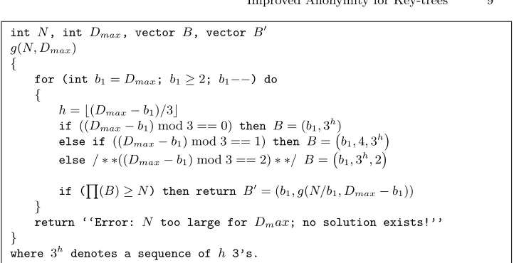
b ≥N, there is at least one solution. The obvious way to find the branching factors of the lexicographically largest solution, is to take agreedy approach. It means that the first branching factor is optimized first, then the second, etc. Algorithm 2 takes N and Dmax as input and solves this problem recursively. Starting from b1 = Dmax, a branching factor b1 is allowed, if a suitable tail (of one of three forms in Theorem 3) can be constructed with the remaining Dmax−b1, such that the product ofBis large enough. If such a tail exists, it is optimized in recursion. If no suitable tail exists,b1 is decremented. If no proper solution can be found at all (for 2 ≤ b1 ≤ Dmax), an error is returned. This means that N is so large that even a binary tree does not allow search within the imposedDmax.
Note that because a tree is constructed only once, during a pre-computation stage, the runtime efficiency of the optimization algorithm is neither essential nor related to the authentication time. However, we note that the complexity of both Butty´an’s algorithm and Algorithm 2 is linear (in N and/orDmax).
Since our search space is larger than Butty´an’s, our optimal branching vector will either be equal to, or lexicographically larger than the output of Butty´an’s algorithm, thus providing better anonymity. The potential difference in output can be illustrated with the help of the following examples:
int N, int Dmax, vector B, vector B′
g(N, Dmax) {
for (int b1=Dmax; b1≥2; b1−−) do {
h=⌊(Dmax−b1)/3⌋
if ((Dmax−b1) mod 3 == 0) then B= (b1,3 h
) else if ((Dmax−b1) mod 3 == 1) then B= b1,4,3
h else /∗ ∗((Dmax−b1) mod 3 == 2)∗ ∗/ B= b1,3
h
,2
if (Q(B)≥N) then return B′= (b
1, g(N/b1, Dmax−b1)) }
return ‘‘Error: N too large for Dmax; no solution exists!’’ }
where 3h
denotes a sequence of h 3’s.
Algorithm 2: Finding an optimal B for Problem 2
larger, although not much. Here, we also see that the tail of ourBmay contain a single element of 5; this shows that recursion is indeed required for our algorithm to always find an optimal solution.
– In Set 2, the input contains relatively large primes. Butty´an’s algorithm cannot improve upon the Classic tree at all, leaving much room for improvement by Algorithm 2. The difference in performance is about as large as between the Classic and Butty´an trees in Set 1.
– For Set 3, Butty´an’s algorithm and Algorithm 2 perform similarly and yield the same output.
Table 1.Test cases
Input Classic Butty´an Optimized Butty´an Set 12
:N= 27000, (30,30,30) (72,5,5,5,3) (73,5,3,3,3,3) Dmax= 90 R= 0.9355 R= 0.9725 R= 0.9729(N′= 29565)
Set 23
:N= 24389, (29,29,29) (29,29,29) (84,4,3,3,3,3), Dmax= 100 R= 0.9333 R= 0.9333 R= 0.9764(N′= 27216)
Set 34
:N = 1728, (12,12,12) (24,4,3,3,2) (24,4,3,3,2) Dmax= 36 R= 0.98462 R= 0.9194 R= 0.9194
2
Butty´an’s example
3
Example with prime numbers
4
3.1 Consequences of Larger Trees
Algorithm 2 can lead to trees that exceed the strictly required number of leaves (withN′ > N). We argue that this has practical advantages, but should also be
taken into account when judging the anonymity of such trees.
A larger tree will allow for addition of tags at a later time, which may be desirable in practice. Ideally, creating and balancing a tree should be done only once, and therefore the tree should accommodate all the tags ever expected to
enter the system. In systems where growth is anticipated, having a larger tree
that is ready for the future is good practice.
Also, since we are defending against tampering attacks, replacement of com-promised tags should be taken into consideration. Replacement tags should
con-tainnew key material, lest they be reintroduced with keys that are already fully
disclosed (immediately limiting their anonymity). Having unused leaves in the tree seems ideal for this purpose.
When choosingwhich leaves to actually use as tags (initially and for replace-ments), we suggest to select a sufficient number of branches at the level d−1
at random, and to randomly initialize tags from these branches. This to create
a subtree of initialized tags that is as close to the original (optimal) shape as possible, without introducing order in the system which might be exploited.
Finally note that tags corresponding to unused leaves in the tree cannot be encountered by adversaries in the field. For this reason, they do not contribute to the size of the set among which targets need to be distinguished. This means that (some) anonymity sets will appear larger than they are in actuality. Because our anonymity measures are all based on set sizes, to prevent overestimating the results of our solution, we apply corrections as detailed below.
Theorem 4.If N tags are placed uniformly at random in a tree with Q(B) = N′ > N, then the expected resistance to c member compromise (Rc) equals
N
N′Rc(B).
Proof. Consider a particular choice ofN tags within the set {ti |1≤i≤N′}.
Consider a particular choice ofc compromised tags within theN tags. Let 1≤
i≤N′. ThenP(ti) denotes the anonymity set of tagti, considering only theN
chosen tags. Note thatP(ti) will be empty when tagtiis not one of theNchosen tags. On the other hand,P′(ti) denotes the anonymity set of tagti, considering
allN′ elements.
It is clear that, when averaging over all possible choices ofN tags, and all possible choices ofccompromised tags,
E[|P′(ti)|] = N
′
N ·E[|P(ti)|]
Therefore,Rc= ¯Sh−i(c)/N =E[N1 PN
i=1
|P(ti)|
N ], which equalsE[ 1 N
PN′ i=1
|P(ti)|
N ], because P(ti) is empty when tag ti was not chosen. Consequently, Rc = E[1
N PN′
i=1
|P′(ti)|
N′ ] =
N
3.2 Simulation forc >1
Section 3 has already shown that our proposal can yield lexicographically larger B than Butty´an’s approach, and consequently better anonymity measures when c= 1. Forc >1, the theoretical analysis becomes very complex, so we compare our approach to Classic and Butty´an trees by means of computer simulations. Both Butty´an and our proposal assume a maximum allowed authentication delay, and try to provide optimal privacy within this boundary. Therefore, it is sensible to compare theanonymity of the two solutions, but not their efficiency (in terms of authentication delay), because both solutions are constructed based on the same maximum authentication delay Dmax.
We will calculate ¯S0(c) and ¯Sh−i(c).Using code written in C++, we iterate
over all possible scenarios in an efficient way, making use of the fact that many scenarios are equivalent with regard to set sizes. The minimum and (weighted) average of ¯S taken over all these scenarios is stored as output. Because the number of scenarios grows rapidly as the number of compromised tags increases, we limit ourselves to cases with 1≤c≤100.
For trees withN′> N, results are corrected by scaling down as discussed in
Section 3.1.
Table 1 shows the three input sets for which we have evaluated the Classic, Butty´an and Optimized Butty´an trees. The following figures provide a graphical comparison of the performance of different trees under various conditions. A selection of the most relevant datasets was made, and some of the figures show partial graphs to provide the required level of detail. We will discuss how these results relate to our hypotheses and claims.
0 10 20 30 40 50 60 70 80 90 100
0 0.5 1 1.5 2 2.5
3x 10 4
number of compromised membersc
a
v
er
age
se
t
si
ze
¯S0
Classic Buttyan
Optimized Buttyan (scaled)
0 10 20 30 40 50 60 70 80 90 100 0
0.5 1 1.5 2 2.5x 10
4
number of compromised membersc
a
v
er
age
se
t
si
ze
¯S0
Classic / Buttyan
Optimized Buttyan (scaled)
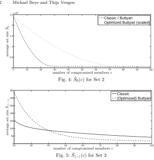
Fig. 4: ¯S0(c) for Set 2
20 30 40 50 60 70 80 90 100
0 50 100 150 200 250 300 350
number of compromised membersc
a
v
er
age
se
t
si
ze
¯S<
−
>
Classic
(Optimized) Buttyan
Fig. 5: ¯Sh−i(c) for Set 3
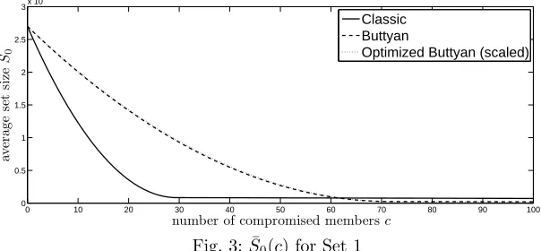
For Set 1, the Optimized Butty´an trees seemed to outperform the regular Butty´an tree significantly in terms of ¯S0(c). However, after correction (to ac-count for the fact thatN′ > N), there is little difference in actual performance
(Figure 3). The same trend was observed for Sh−i(c), and the result for Set 3
(not displayed here). We note that the performance of the Optimized Butty´an trees in no case drops below that of the original Butty´antrees.
Results for Set 2 differ, because the Butty´an tree there is strongly suboptimal in shape, with Figure 4 clearly showing the advantage of the Optimized Butty´an tree. This is due to the fact that the chosen N has too few prime factors for Butty´an’s algorithm to work with. In similar cases, the same problem will occur to a greater or lesser extent.
Based on Figure 5, we observe a turning point where the classic tree starts to outperform the (Optimized) Butty´an trees. This occurs in all graphs, at c=b1 for ¯S0 and atc ≈b1 forSh−i. At these points, the decrease of ¯S slows causing
[is expected to have been] broken down, because each top-level branch contains [can be expected to contain] at least one compromised tag. Because subsequent compromised tags then fall into smaller sets, the adversary will learn little new information; he has obtained the most important keys in the tree already. In such a worrying scenario, what little anonymity tags have left depends upon the keys in lower branches. Classic trees retain slightly more anonymity, because they have larger branching factors at the bottom levels. However, given the (by then) minimal values of ¯S overall, theabsolute advantage is not large.
4 Conclusions and Future Work
Our proposed Algorithm 2 yields better results than Butty´an’s original approach, when it comes to finding the lexicographically largestB. We have provided proof that the solution is optimal in terms of optimization problem 2. The output is at least as good (often superior, in some cases identical) to Butty´an trees in terms ofR, ¯S0(c) and ¯Sh−i(c).
Algorithm 2 can result in trees withN′≥N, which may be advantageous in
growing systems or when replacing compromised tags. It also means that care must be taken not to overestimate the anonymity, leading us to apply corrections to our simulation results. The corrected results still clearly show the advantage of our tree construction to both Classic and Butty´an trees.
Future work:
We wish to expand our current results, by taking side-channel knowledge and adaptive adversaries into consideration. A paper detailing the results of this has recently been accepted at the SecureComm2011 Conference [3]. Defending against adaptive attacks leads to a different optimization problem (and a differ-ent optimal tree shape), and thus to a trade-off between defending against naive and adaptive adversaries. This is related to our observation that anonymity is mostly lost when c ≈b1, and the fact that this process may be accelerated by adversaries who are able to accurately choose which tags they compromise.
As is evident from our examples, Algorithm 2 provides results that are much better, better, or identical to Butty´an’s results, depending on the exact inputs N and Dmax. Additional experimentation could show what the expected gain in anonymity is in the average case (for randomly chosen N and Dmax), thus better illustrating the actual performance of Algorithm 2 in practice.
References
1. Gildas Avoine, Etienne Dysli, and Philippe Oechslin. Reducing Time Complexity in RFID Systems. In Bart Preneel and Stafford Tavares, editors, Selected Areas
in Cryptography – SAC 2005, volume 3897 of LNCS, pages 291–306, Kingston,
Canada, August 2005. Springer-Verlag.
2. Gildas Avoine, Pascal Junod, and Philippe Oechslin. Time-Memory Trade-Offs: False Alarm Detection Using Checkpoints, Extended Version. Technical report, 2005. LASEC-REPORT-2005-002.
3. Michael Beye and Thijs Veugen. Anonymity for key-trees with adaptive adver-saries, 2011. Accepted at SecureComm2011, 7th International ICST Conference on Security and Privacy in Communication Networks.
4. Levente Butty´an, Tam´as Holczer, and Istv´an Vajda. Optimal Key-Trees for Tree-Based Private Authentication. InIn Proceedings of the International Workshop on
Privacy Enhancing Technologies (PET), June 2006. Springer.
5. Ivan Damg˚ard and Michael Østergaard Pedersen. RFID Security: Tradeoffs be-tween Security and Efficiency. Cryptology ePrint Archive, Report 2006/234, 2006. 6. Claudia D´ıaz. Anonymity Metrics Revisited. In Shlomi Dolev, Rafail Ostrovsky, and Andreas Pfitzmann, editors,Anonymous Communication and its Applications, number 05411 in Dagstuhl Seminar Proceedings. Internationales Begegnungs- und Forschungszentrum fuer Informatik (IBFI), Schloss Dagstuhl, Germany, 2006. 7. Hannes Federrath, editor. Anonymity, Unobservability, and Pseudonymity - A
Proposal for Terminology, volume 2009 ofLNCS. Springer-Verlag, 2001.
8. Tamas Holczer Istvan Vajda Gildas Avoine, Levente Butty´an. Group-based private authentication. InIEEE International Symposium on a World of Wireless, Mobile
and Multimedia Networks, pages 1–6, 2007.
9. M. Hellman. A cryptanalytic time-memory trade-off. InInformation Theory, IEEE
Transactions on, volume 26, pages 401–406, July 1980.
10. Ari Juels and Stephen A. Weis. Defining Strong Privacy for RFID. InPERCOMW ’07: Proceedings of the Fifth IEEE International Conference on Pervasive
Com-puting and Communications Workshops, pages 342–347, Washington, DC, USA,
2007. IEEE Computer Society.
11. David Molnar and David Wagner. Privacy and security in library RFID: issues, practices, and architectures. InCCS ’04: Proceedings of the 11th ACM conference
on Computer and communications security, pages 210–219, New York, NY, USA,
2004. ACM.
12. Yasunobu Nohara, Toru Nakamura, Kensuke Baba, Sozo Inoue, and Hiroto Ya-suura. Unlinkable identification for large-scale rfid systems.Information and Media
Technologies, 1(2):1182–1190, 2006.
13. Karsten Nohl and David Evans. Quantifying information leakage in tree-based hash protocols (short paper). In Peng Ning, Sihan Qing, and Ninghui Li, editors,
ICICS, volume 4307 of LNCS, pages 228–237. Springer, 2006.
14. Miyako Ohkubo, Koutarou Suzuki, and Shingo Kinoshita. Cryptographic Ap-proach to “Privacy-Friendly” Tags. InRFID Privacy Workshop, MIT, MA, USA, November 2003.
15. Stephen A. Weis, Sanjay E. Sarma, Ronald L. Rivest, and Daniel W. Engels. Security and Privacy Aspects of Low-Cost Radio Frequency Identification Systems. In Dieter Hutter, G¨unter M¨uller, Werner Stephan, and Markus Ullmann, editors,
16. Sang-Soo Yeo and Sung Kwon Kim. Scalable and Flexible Privacy Protection Scheme for RFID Systems. In Refik Molva, Gene Tsudik, and Dirk Westhoff, edi-tors,European Workshop on Security and Privacy in Ad hoc and Sensor Networks
– ESAS’05, volume 3813 ofLNCS, pages 153–163, Visegrad, Hungary, July 2005.
Springer-Verlag.
A Proof of Theorem 2
The first observation is that for an optimalB,P
(B) =Dmax, otherwiseDmax−
P
(B) could be added to any element of B without violating the constraints while increasing R(B). So we assume P
(B) = Dmax in the proof, which uses four Lemmas, similar to the Lemmas of Butty´an’s work [4]. It’s also clear that an optimalB will have branching factors at least 2. The first Lemma, Lemma 1, shows that a branching vector can always be improved by ordering its elements in decreasing order. Lemma 3, using some bounds from Lemma 2, shows that given two branching factor vectors, the one with the larger first element is always at least as good as the other. Lemma 4 generalizes Lemma 3 by stating that given two branching factor vectors the first j elements of which are equal, the vector with the larger (j+ 1)-st element is always at least as good as the other.
These Lemma’s together show that a lexicographically larger branching factor vector will always be at least as good as the lexicographically smaller branching factor vector (in caseP
(B) =Dmax), so indeed the solution with maximalR(B) to Problem 2 is achieved by the lexicographically largest vector that satisfies the constraints.
Lemma 1.Let B be a branching factor vector, and let B∗ be the vector that
consists of the sorted permutation of the elements ofB in decreasing order. IfB
satisfies the constraints of Problem 2, thenB∗ satisfies them too, andR(B∗)≥
R(B).
Proof. SinceQ
(B) is not altered by the permutation, we can refer to Butty´an’s proof [4] of Lemma 1. ⊓⊔
Lemma 2.Let B = (b1, . . . , bd) be a sorted branching vector (i.e. b1 ≥ b2 ≥ . . .≥bd). We can give the following lower and upper bounds onR(B):
1− 1
b1 2
≤R(B)≤R(b1) =1 + (b1−1) 2
b2 1
Proof. The lower bound is identical to Butty´an, hence the proof [4] is as well.
The upper bound is an improvement w.r.t. Butty´an, and is proven as follows. LetM =Q(B), thenQ(B\bd) =M/bd. We derive ford >1:
R(B) = 1 M2
1 + (bd−1)2+ d−1 X i=1
(bi−1)2 d Y j=i+1
= 1 M2
1 + (bd−1)2+ d−2 X i=1
(bi−1)2 d Y j=i+1
b2j+ (bd−1−1)2b2d
=R(B\bd)− b
2 d
M2 1 + (bd−1−1) 2
+ 1
M2 1 + (bd−1) 2+ (bd
−1−1)2b2d
=R(B\bd) +2−2bd M2 < R(B\bd)
and by recursively applying this inequality alsoR(B)≤R(b1). ⊓⊔
Lemma 3.Let B = (b1, . . . , bd) andB′ = (b′1, . . . , b′d′)be two sorted branching factor vectors (i.e. b1 ≥ b2 ≥ . . . ≥ bd, b1′ ≥ b′2 ≥ . . . ≥ b′d′) that satisfy the constraints of Problem 2. Then,b1> b′1 impliesR(B)≥R(B′).
Proof. We first prove the statement forb′
1≥3. From Lemma 2 we know that
R(B′)≤ 1 + (b
′
1−1)2 b′
1 2
and
R(B)≥
1− 1
b1 2
>
1− 1
b′
1+ 1 2
which follows from the fact that b1 > b′1. A straightforward calculation shows that (1− 1
b′
1+1)
2≥1+(b′1−1)2 b′
1
2 wheneverb′1≥3, and thusR(B)≥R(B′).
So the remaining case isb′
1= 2. SinceB′ is ordered, each element ofB′ will equal 2. If d′ = 1 then by our previous assumption Dmax = P
(B′) = 2, but this contradicts Dmax =P(B)≥3, so we know d′ ≥2. The resistance R(B′)
is readily computed as R(B′) = 1 3(2·4
−d+ 1), which will be at most 3 8 (when d′= 2). SinceR(B)≥(1− 1
b1)
2>(1−1 3)
2=4
9, it follows that also in this case R(B)≥R(B′). ⊓⊔
Lemma 4.Let B = (b1, . . . , bd) andB′ = (b′1, . . . , b′d′)be two sorted branching factor vectors (i.e. b1 ≥ b2 ≥ . . . ≥ bd, b1′ ≥ b′2 ≥ . . . ≥ b′d′) that satisfy the constraints of Problem 2. Let j, 1≤j < min(d, d′), be such thatbi =b′i for all i,1≤i≤j, andbj+1> b′j+1, thenR(B)≥R(B′).
Proof. It is easy to show thatR(B) =b1−b11
2 +b12
1·R(B\b1). Therefore, since b1 = b′1, R(B) ≥ R(B′) whenever R(B\b1) ≥ R(B′\b′1). By recursively ap-plying this rule, and using Lemma 3, which shows that R(B\{b1, . . . , bj}) ≥ R(B′\{b′