Reasoning with Non-Numeric Linguistic Variables

Reasoning with Non-Numeric

Linguistic Variables

Jon Williams, Nigel Steele and Helen Robinson

Computational Intelligence Group, School of Mathematical and Information Sciences, Coventry University

Where decisions are based on imprecise numeric data and linguistic variables, the development of automated decision aids presents particular difficulties. In such applications, linguistic variables often take their values from a pre-ordered set of vaguely defined linguistic terms. The mathematical structures that arise from the assumption that sets of linguistic terms are pair-wise tolerant are considered. A homomorphism between tol-erance spaces, filter bases and fuzzy numbers is shown. A proposal for modeling linguistic terms with an ordered set of fuzzy numbers is introduced. A procedure for structured knowledge acquisition based on the topology of the term sets and the cognitive theory of prototypes is shown to give rise to sparse rule bases. Similarity as a function of “distance” between fuzzy numbers treated as tolerance mappings is used as an inference mechanism in sparse rule bases to give linguistically valued outputs. Measuring the “distance” between fuzzy sets to correspond to intuitive notions of nearness is not straightforward, since the usual metric axioms are not adequate. An alternative way of measuring “distance” between fuzzy numbers is introduced, which reduces to the usual one when applied to crisp numbers.

Keywords: linguistic variables, tolerance spaces, fuzzy numbers, similarity based reasoning.

1. Introduction

There is a particular class of problems which have a small set of mutually exclusive decision outcomes where the development of automated decision aids presents particular difficulties. In these domains decisions are based on both im-precise numeric data and linguistic variables which have no underlying numeric scale. (A very simple example is deciding whether a stu-dent should pass or fail a course based on their mark and performance in seminars. The mark is imprecise because of marker variation and per-formance in a seminar takes a linguistic value

such ascompetent). These decisions tend not to have well defined rule sets, making traditional expert systems difficult to develop.

There is a substantial body of work dealing with linguistic variables and their modeling with fuzzy sets. It is Zadeh’s contention that Fuzzy logic = Computing with wordsZadeh 1996]. However, in applications, fuzzy sets and fuzzy logic are most often applied to variables which have an underlying numeric scale. Modeling non numeric linguistic variables is acknow-ledged to be less well developed.(For example by Cox on who wrote in thecomp.ai.fuz|zy

newsgroup on 28 March 1999“The application of fuzzy logic and fuzzy metrics to non-numeric objects (and events) has long been a difficult task”.)

this paper, we show how alternative, but es-sentially equivalent mathematical structures of

filter basesandtolerance spaces, provide a pos-sible solution to this problem. The approach taken here is designed to deal with problems where the only variables are non-numeric and also to combine non-numeric variables with nu-meric variables. In both cases it is possible to give imprecise linguistic outputs which convey the uncertainty of outcomes to a user in an in-tuitive way.

Definition 1. (Non-Numeric Linguistic Vari-able) A non-numeric linguistic variable is cha-racterised by a quintuple hv L X g mi; in which v is the name of the variable; L is a

finite set of linguistic terms fl0 ::: lng which describe v whose states range over a universal set X of states of v; g is a grammar for gene-rating linguistic terms, and m is a semantic rule which assigns to each term l 2 L its meaning m(l)on X; that is m :L!AX.

Example 1. Consider the performance of a student in a seminar. Thenv = seminar. The set Xseminar of possible states of a student’s performance ranges from no contribution to

superb. These states are described by a pre-ordered set Lseminar with a grammar (g) of at least three terms, for examplefpoor competent

goodg. The grammar (g) might also specify how many additional terms may be added. So for example the termsvery poorandvery good

might be added. (The number of terms used in applications is discussed in section 6.2.). Thenm(poor)maps to the lower portion of the seminar performance range so thatm(poor) m(competent).

Definition 2. (Numeric Linguistic Variable)

A numeric linguistic variable is characterised by a quintuplehv L X g mi;inwhich v names the variable; L is afinite set of linguistic terms

fl0 ::: lng of the base variable v whose val-ues range over a universal set X of valval-ues of v; g is a grammar for generating linguistic terms; and m is a semantic rule which assigns to each term l 2 L its meaning m(l)on X, (i.e. m(l):L!AX).

Example 2. Consider the marks gained by a student on a course. Then v = mark. The setXmarkof possible values of a student’s mark

range from 0 to 100. These states are described by a pre-ordered setLmark with a grammar(g) of at least two terms, for exampleffail,passg. Again the grammar might also specify how ad-ditional terms were to be added. (So, for exam-ple, the term marginal pass may be added). Then we could have m(fail) = 0 40) and m(pass) = 40 100]. We might also have m(marginal pass) = (35 45] if it is possible to pass with a mark less than 40, but not with a mark less than 35.

2. Sets of Linguistic Terms — Mathematical Structure

In this section assumptions will be made about the mathematical structure of sets of linguistic terms. The following definitions are required.

2.1. Orderings

Definition 3. (Preorders) Let A be a set, then whenever there is a defined concept of less than or equal to then this establishes a pre-order on A [Nachbin 1965]. More formally, a preordered set is a set A equipped with a reflexive transitive operation such that if a b c2A then a a (reflexivity) and in addi-tion a b and b c implies a c (transitiv-ity).

Definition 4. (Partial Orders and Chains)

A partial order is a preorder where in addi-tion satisfies a b 2 A then a b and b a implies a = b. A partial order relation is linearly ordered or a chainif

8a b2A either ab or ba:

Definition 5. (Up sets) Let P be a partially ordered set with Q P. Then Q is an up set whenever x 2 Q, y 2 P and y x then y 2 Q. If x is the least element in Q then the set is often referred to as the up set of x. Down sets are defined by duality. The up set of x is denoted"x and the down set of x by#x.

Example 4. The set of pairsf(m n):(m n)2 N Ng with (m1 n1) (m2 n2) , m1 m2&n1n2is a partial order, but not a chain, since(4 3)is not comparable with(3 4).

2.2. Vague Linguistic Terms

The remainder of this paper is based on the following assumptions about the sets of vague linguistic terms which are used to valuate vari-ables in decision making environments. Let a finite set of mutually exclusive decisionsD := d1 ::: dn have a finite set p 2 N of attributes described by a finite set of linguistic variables V :=v1 ::: vp.

Preorder

Eachvktakes a value or range of values from a finite pre-ordered set of linguistic terms value: V ! L to give value(vk) = li, (0 i card(L)) and the pair hli vki which we will denoteli vk.

Example 5. For the variable mark we have the linguistic variablespassmark andfailmark.

Kernels

Assume for eachli vk there is at least one state

ofvkto which only that term applies, thekernel ker(li v

k)of the term, so that m(ker(li))

\

m(ker(li +1

))=

for eachli2L.

Example 6. For the term set

fpoor competent goodgseminar

there exist states which are only mapped to one term so that the strict precursor relation

ker(poor)ker(competent)ker(good) holds and the meaningsm(see definition 1)are disjoint

m(ker(competent))\m(ker(good))=:

Pairwise tolerance

We assume that vague linguistic terms are pair-wise tolerant so that

li vk\li +1vk

=τR(li v

k)=τL(li +1vk

)6= the meaning m : Lvk ! Xgivesm(τR(li)) = m(τL(li

+1

)). HereτRis theright toleranceand

τLthe left tolerance. The least element of Lvk

is assumed to have no left tolerance and the greatest element no right tolerance. Note that

τL(li)<ker(li)<τR(li).

Example 7. The termpoorcompetent =)

m(poor)\m(competent)6=.

Support

Taking the previous two assumptions together, assume that each linguistic term has as asupport set the points supp(li)=fτL(li) ker(li) τR(li)g so thatm(supp(li))=m(li).

Pairwise concatenation

The operation of concatenation of the lin-guistic terms li lm 2 Lv

k is defined pairwise.

So that

li m =li:::lm = m

i

lj (ijm)

which is the same as

li m =f"li\#lm:li<lmg: This is equivalent to the logicalOR‘W

’ opera-tion. Note that

ker(li m)=fker(li) τR(li) ::: τL(lm) ker(lm)g:

Example 8. For a variablev0described by the

term set

fvery bad-bad-medium

-good-verygoodgv

0

then

very badv0mediumv

0 =

fvery bad, bad, mediumgv

0

which may be read fvery badv

0 _badv

0 _mediumv

Products

The productQ

of two sets of linguistic terms is defined on the product space of their respective variablesvk vjto give the pairli v_k li vjand

nat-urally extended toQp

1vkto give(li v

1 li v

p).

Example 9. For two variablesv1=markand v2 =seminarwe have the product spacemark

seminar. A range of numerical values35, 45] of mark may be described by the term

marginal pass, and range of states of semi-nar by the term competent. Then the pair of terms(marginal passmark,competentseminar), can be read

fmarginal passmarkandcompetentseminarg

3. Mathematical Structures and Linguistic Variables

AlbrechtAlbrecht 1998]draws attention to the fact that many elements of knowledge-based systems and uncertain reasoning can be cap-tured by traditional mathematics and, in par-ticular, by topology. Hovesepian Hovesepian 1992]shows that a tolerance space is sufficient to model the sorites paradox using a three val-ued logic and StoutStout 1992]considers the relationship between tolerance spaces and fuzzy sets in a category theoretic setting.

Definition 6. (Topological Space – Open Sets)

Atopologyon set X is a collectionT of subsets of X with the following properties:

O1 X2T and2T.

O2 The union of any number of sets in T be-longs toT.

O3 The intersection of any two sets in T be-longs toT.

The pair(X T)is called atopological space.

Definition 7. (Open sets) Members ofT are called open sets. The complement of an open set isclosed. An alternative, equivalent, defi ni-tion of a topology may be phrased in terms of closed sets [Kelley 1955].

Definition 8. (Bases) Let(X T)be a topolog-ical space. A base forT is a collectionBT such that every set inT is a union of sets from

B.

Definition 9. (Sub-bases) A sub-base for a topologyT is a collectionS T such that any set inT is a union offinite intersections of sets fromS.

It will be shown later that if the supports of linguistic terms(i.e. fτL(li) ker(li) τR(li)gare taken as a sub-base for a topology, then the ker-nels ker(li)are closed.

Different topologies have different separation propertiesKelley 1955]described by theTi ax-ioms two of which we will require.

Definition 10. A topology on(X T)is:

T2 or HausdorffIf and only if, given a pair of

distinct points x y of X there exist open sets

OandO

0with x

2Oand y 2O

0, such that

O\O 0

=.

T0 If for each distinct x and y in X, there exists

an openO2 T such that either x 2O and y 62 O, or there exists O

0

2 T, such that y 2O

0

and x 62O 0

.

Equivalently a topology is T0 if and only if,

given a pair of distinct points x y of X there exists an open setO, such thatO\fx ygis a singleton.

Definition 11. (Tolerance Relation) A toler-ance relation is a symmetric reflexive relation

ξ X X, such that xξx for every x 2 X and xξy =) yξx for all x y 2X.

Definition 12. (Tolerance Space – [Zeeman 1962]) Atolerance space,hX ξiis a space X with a tolerance relationξ 2 X X, the tole-rance on X. Ifhx yi2 ξ denoted xξy, then x is said to be within ξ tolerance of y. A space may be equipped with more than one tolerance. A bi-tolerant space is a spacehX hξ ζiiwith

ξ ζ δ, whereδ is the discrete tolerance and xδy ,x =y. In a tolerance spacehX ξi the set N(x)fy:yξxg, is called at-neighborhood of x 2 X. The t-neighborhood of a subset A of X is the union of the t-neighborhoods of all its points, that is

N(A)=

Example 10. Take r1 r2 2 R and let r1ξr2

() jr1;r2j<1; then N(r1) =(r1;1 r1+1). Now take1 2]R; then N(1 2])=(0 3): A topological space (X T) is tolerable Ho-vesepian 1992] if there exists a ξ on X, such that the setfN(x): x 2 Xgof t-neighborhoods serves as a sub-basis for a topologyT onX.

Example 11. Consider the relation described in example 10; the set fN(r) : r 2 Rg is a sub-basis for the usual topology.

Example 12. Consider the set of neighbor-hoodsfN(1) N(2)gwith the tolerance relation defined in example 10. Then they generate a topology onN(1 2])given by

f(0 3) (0 2) (1 3) (1 2) g:

Definition 13. (Tolerance Mapping) Let f : hX ξi!hY ζibe a map between two tole-rance spaces then f is a toletole-rance map, if

xξy 2hX ξi =) f(x)ζf(y)2hY ζi:

If the converse holds, then f is atolerance em-bedding.

3.1. Topologies of Linguistic Terms

Different approaches can be taken to topologies of the term set of a linguistic variable. The sup-ports of the linguistic terms can be taken as a sub-base for a topology. On the other hand, the kernels and tolerances may be taken as a base for a topology which gives a different topology with different, but related separation properties. It is also possible to define a topology by tak-ing the (concatenated) kernels alone as a ba-sis for the closed sets. The difference in the nature of these spaces is important; since em-pirical evidenceZwick 1988, Yoshikawa 1996] suggests that people judge the similarity of lin-guistic terms on the basis of the separation of the kernels of the terms.

Theorem 1. Let S =

S i2I

supp(li)be the set of tolerances and kernels for the kth _linguistic variable. Then the topology Ls on S obtained by takingfsupp(li)gi

2I as a sub-base is T0 but not T2.

Proof. Sets of the formfτL(li) ::: τR(li)gare open in(S Ls).

Every open set which contains ker(li)also con-tainsτL(li) = τR(li

;1 ) 2 li

;1 hence

(S Ls) is notT2.

Take ker(li) ker(lj) or τ(li) τ(lj) as distinct points, then there are open setsliandτ(li)such thatli\fker(li) ker(lj)gandτ(li)\fτ(li) τ(lj)g are singletons. Taking ker(li) τ(lk)thenτ(lk)\ fker(lj) τ(lk)g=τ(lk)is a singleton and(S Ls) isT0.

Theorem 2. Let S =

S i2I

supp(li). Then the topology(S Lk)obtained by taking the concate-nated kernels K =fker(li j): i2Igas a base is T0but not T2.

Proof. ker(li) τR(li) are distinct points not in disjoint sets since τR(li) 2 ker(li i

+1 ) and ker(li)\ker(li i

+1

) 6= hence (S Lk) is not T2. Every member ofLkwhich contains ker(li) also containsτL(li)orτR(li

+1

)hence(S Lk)is T0.

Theorem 3. Take S as in theorems 1 andLp=

ffτL(li)g fker(li)g fτR(li)g:i2Igas a basis for a topology on S then(S Lp)is Hausdorff.

Proof. The τ(li) are open and disjoint, both from each other and the ker(li). Similarly the ker(li)are closed and disjoint, both from each other and theτ(li).

The topology (S Lp) is also T0 since all T2 spaces areT0 Kelley 1995], however the con-verse does not hold.

It follows that the topology on the product space (S Ls)obtained by taking the partially ordered set

Ls = n Y

k=1 Lvk =

n Y

k=1 fli v

kg

as a sub-base is not Hausdorff. However the topology given by (S Lp) obtained by taking as a basis the partially ordered set

Lp= n Y

k=1 Pvk =

n Y

k=1 fpi v

wherepiis theithelement in the chain ker(l0)<τR(l0)<:::τR(ln

;1

)<ker(ln) is Hausdorff. Since all metric spaces are Haus-dorff these results suggest that a metric space may be an inappropriate model for the term sets of linguistic variables. There is, however, a continuous mapping φ : (S Lp) ! (S Ls) between the two spaces such that

φ(ker(li +j v1

) ker(li +j vk

))7!

(li +j v1

li +j vk

) (0i jjLj;1) which means that it is possible to work in the Hausdorff space (S Lp) and map into the T0 space(S Ls)or to work with the bi-topological space (S hLs Lpi)and so move between the strictlyT0spaces of the linguistic terms and the

T2space of the disjoint kernels and tolerances.

3.2. Filters and Filter Bases

It is convenient to introduce here the concepts ofFiltersandFilter Bases.

Definition 14. (Filter Base) A non empty sys-tem B of subsets of the set X is called a filter basison X if the following conditions are

satis-fied.

FB1 the intersection of any two sets from B contains a set fromB.

FB2 the empty set does not belong toB.

Example 13. For any a > 0 x 2 R; B = ffxg x;a x+a]gis a filter base.

Given this definition, we prove the following theorem

Theorem 4. Let l = fli ker(li)g with li =

fτL(li) ker(li) τL(li +1

)gthen l is afilter-base.

Proof. Both FB1 and FB2 are satisfied since: li\ker(li)=ker(li)2 land2= l.

If we add to every set of a filter basis all of its supersets, then FB1 is sharpened and we get a

filter.

Definition 15. (Filter) A non empty systemF of subsets of the set is X is called afilter(on X) if the following conditions are satisfied.

F1 Every superset of a set from F belongs to

F.

F2 The intersection of any two sets fromF be-longs toF.

F3 The empty set does not belong toF.

Note that while every filter is a filter base the converse is not true.

Example 14. For anyai bi x 2R i2 N and ai < bi with a1 > a2 > > an and b1 > b2> >bn thenB =ffxg x;ai x+bi]g is a filter.

Any unconcatenated linguistic term li can be transformed into a filter by introducing the nes-ted sets τL(li) τL

j(li) τL

j0

(li) with

τL_j0

(li) < ker(li) and similarly for fτR

jg > ker(li) j 2 J, an indexing set. Then we can prove

Theorem 5. If l0

= fli ker(li)g with li = ffτL

j(li)g ker(li) fτR

j(li)g :i2 0 jLj;1]j2 J(an indexing set)gthen l

0is afilter.

Proof.F1, F2 and F3 are satisfied since:

fτL

j(li) ker(li) τR

j(li)g fτL

j0

(li) ker(li) τR

j0 (li)g

ker(li) also

fτL

j(li) ker(li) τR

j(li)g \fτL

j0

(li) ker(li) τR

j0 (li)g

=fτL

j0

(li) ker(li) τR

j0

(li)g2l 0

and

ker(li)\fτL

j(li) ker(li) τR

j(li)g=ker(li)2l 0

and finally2= l 0

Theorem 6. Let S = S

i2I

supp(li) then the topology(S Lf)obtained by taking

F =ffτL

j(li) ker(li) τR

j(li):j2Jg:i2Ig as a sub-base is T0but not T2.

Proof. Take p 2 τR

j(li)then there is no j 2 J such thatpand ker(li)are in disjoint open sets; hence(S Lf)is notT2.

Consider W1 = fp1 p2 : p1 6= p2g such that p1 p2 2 τL(li) then W1 \ τL

j(li) is a single-ton for some j 2 J, a similar argument ap-plies to p1 p2 2 τR(li). Next consider W2 = fp1 ker(li) :p16=ker(li)gsuch thatp1 2τL(li) or p1 2 τR(li), thenW2\τL(li)orW2\τR(li) are a singletons. Now take W3 = fp1 p2 : p1 6= p2gsuch that p1 2 τL(li)and p2 2 τR(li) then W3 \ τL(li) is a singleton. Finally take W4 = fker(li) ker(li

0)g then W4

\supp(li) is a singleton. Hence given any pair of distinct points p1 p2 of S there exists an open set O, such thatO\fp1 p2gis a singleton and(S Lf) isT0.

4. Filter Bases and Fuzzy Sets

In this section we show how filter bases are related to fuzzy sets. Before doing so, two pre-liminary definitions are needed.

Definition 16. (Proper Filter Base) A filter base isproperifT

B6=.

Definition 17. Let f : X ! Y then f is a -homomorphismif8a b2X ab implies f(a) f(b). If f preserves meets and joins so that f(a_b) = f(a)_ f(b) and f(a^b) = f(a)^ f(b)then f is alattice homomorphism [Davey and Priestley 1990].

Albrecht Albrecht 1998] shows that given a proper filter base such that B = fBj : j 2 Jg on hP(B) \ia non-empty latticehC u tiand a-homomorphismφ :P(B)!C with cj = φ(Bj) then fcjg = φ(B) is a filter base onCif allcj6=andφ(limB)limφ(B). Where limB =

T j2J

Bj and limφ(B) = T

j2Jφ (Bj):

Now considerφ;1 : C

! P(B) defined for all c 2 C byφ

;1 (c) :=

S

φ(U)=c

U. Then φ;1 is a lattice homomorphismBourbaki 1967].( Re-quiringBto be a proper filter base ensuresφ

;1 is well defined sinceφ;1

(c)6= 8c2C.) If C = fcl : l 2 Lg is a filter base on C and for all c 2 C φ

;1

(c) 6= then φ ;1

(C) is a filter base onP(B). In the function(Bj cj)j

2J the elementsBj of a filter base B with support B=

S

Bare valuated bycjwithcj=φ(Bj).

Definition 18. (Fuzzy Set) Zadeh defines [Zadeh 1965] a fuzzy subset A of a set X as a nonempty subset

A=f(x µA(x)):x 2Xgof X 0 1] for some functionµA :X !0 1]: The common practice of referring to fuzzy sub-sets as fuzzy sub-sets will be adopted from now on. The alpha-level set of a fuzzy set A_α on X is defined as

A_α =fx 2X :µA(x)α for eachα 2(0 1]g Thesupportof a fuzzy set is given by

A₀+ =fx 2X:µA(x)>0g and thekernelof a fuzzy set by

A1=fx 2X :µA(x)=1g

Fuzzy subsets ofR are often referred to as fuzzy numbers or fuzzy intervals and are defined as follows:

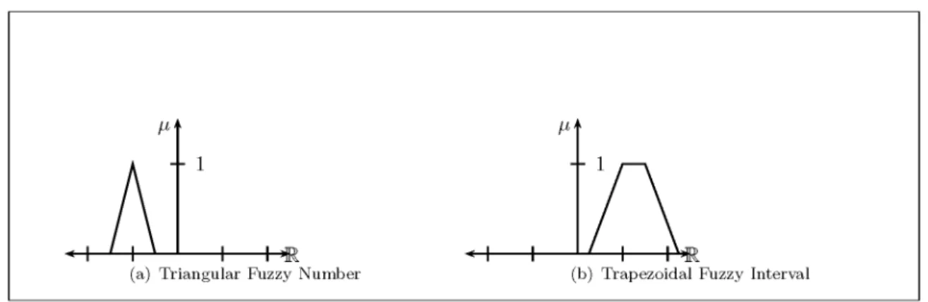
Definition 19. [Goetschel 1983]Afuzzy num-berorfuzzy intervalis a fuzzy set with member-ship function

µ :R !I =0 1]with the properties: 1. µ is upper semi-continuous.

2. µ(x)=0outside some interval(a d)2R. 3. there are b and c2 R with a b c d,

Fig. 1.Fuzzy Numbers.

Definition 20. A Triangular Fuzzy Number (Figure 1(a))en is characterised by an ordered triple < a1 a2 a3 > with a1 a2 a3 such thaten0+

= (a1 a3)and e

n1 = fa2gor for sym-metrical triangular fuzzy numbers as the toler-ance spaceha2 h

(a3;a1)

2 ii.

Definition 21. ATrapezoidal Fuzzy IntervalIe is characterised by an ordered quadruple

< a1 a2 a3 a4 > with a1 a2 a3 a4 such thateI

0+ = (a1 a4)and e

I1 = a2 a3]. For symmetrical trapezoidal fuzzy intervals they can also be represented as the bi-tolerance space

h (a2;a1)

2 h

(a4;a1)

2

(a3;a2)

2 ii. The mem-bership function describes a trapezoid (Figure 1(b)) since the boundaries of theα-level sets

e

I_α=a2;(1;α)(a2;a1) a3+(1;α)(a4;a3)] are the straight lines joining successive mem-bers of the quadruple. A triangular fuzzy num-ber is a special case of a trapezoidal fuzzy inter-val when a2=a3. Note that allowing the mem-bership function to be semi-continuous permits a1 = a2 = a3 for Triangular Fuzzy Numbers and a1 = a2 = a3 = a4 for Trapezoidal Fuzzy Intervals.

Having introduced the concept of fuzzy sets, we can now show how they are related to filter bases.

Theorem 7. ([Albrecht 1998]) A fuzzy set, fuzzy interval or fuzzy number is a valuatedfi l-ter base.

Proof. Take B = a b] R, with a < b, and C =(0 1]R and a functionµ : B!Cwith

the requirement that9x 2 B : µ(x) = 1. Then define a filter baseC =fα 1]:α 2(0 1]gand B_α := µ

;1

(α 1]) as an alpha-cut. Then the filter base B = fBα : α 2 (0 1]gdescribes a fuzzy set,Bwith membership functionµ. Since fuzzy intervals and fuzzy numbers are fuzzy sets this result applies to them equally.

The support(A0+) and kernel (A1) of a trape-zoidal fuzzy interval are a trivial filter base since A1\A0+ = A1and neitherA1norA0+ is empty.

Theorem 8. A fuzzy set is a sequence of valu-ated neighborhoods in a sequence of tolerance spaces.

Proof. Let hX ξibe a tolerance space, then a toleranceζ is said to be finer thanξ ifξ ζ, the finest tolerance is the discrete toleranceδ

and the space hX δi is the discrete tolerance space where every point is only in tolerance of itself. A neighborhood ofa2X,N(a) N

0 (a) if N(a) 2 hX ξi and N

0

(a) 2 hX ξ 0

i with

ξ ξ 0. So

fNi(a)g:=fNi(a)2hX ξii:ξi ξn δg is a filter base and the result follows from theorem 7.

Taking these two results together with theorem 5 gives the following theorem.

Theorem 9. If l = flj ker(lj)g with lj =

ffτL

i(lj)g ker(lj) fτR

i(lj)gg then l can be rep-resented by a fuzzy set withµl(ker(lj))=1and 0<µl(fτL

i(lj)g) µl(fτR

Proof. Apply theorems 7 and 8.

In section 5 a way of representing a non numeric linguistic term with a fuzzy number or fuzzy in-terval is discussed in detail. The following tra-ditional definition of linguistic variableZadeh 1973]is now justified.

Definition 22. (Fuzzy Linguistic Variable) A fuzzy linguistic variable is characterised by a quintuplehv L X g mi; in which v is the name of the variable, L is afinite set of linguistic terms

fl0 ::: lngwhich describe v whose states range over a universal set X of states of v; g is a gram-mar for generating linguistic terms, and m is a semantic rule which assigns to each term l2L its meaning m(l)which is a fuzzy set on X; (i.e. m(l):L!FX).

An example of student marks shows how a tol-erance mapping may be a better model than a fuzzy one based on the extension princi-ple Zimmerman 1987] or interval arithmetic Moore 1966].

Example 15. Let q be a mark in0 100]2 Q and let there be a variation of5in the marks awarded because of marker variation. Then a mark q can be described as a tolerance mapping to the space h0 100] 5ior as a triangular fuzzy numberqe

=hq;5 q q+5i.

If we wanted to see the effect of adding an ad-ditional marks 10 to a student’s score of 30 then adding the marks 30 + 10 gives 40 5. This is a mapping from h0 100] 5i h0 100] 5i!h0 100] 5iand is equiva-lent to a fuzzy numberh35 40 45i.

However30e +

e

10=h40;10 40 40+10i= h30 40 50i mapping to the triangular fuzzy numbers using the extension principle.

Since the tolerance is known for any mark there is no reason to suppose that it will double if ad-ditional marks are added. This example shows how the tolerance model may capture the intu-itive notions better than the fuzzy one based on the extension principle.

5. Numeric Representations of Non-Numeric Linguistic Variables

In applications we need to represent non-numeric linguistic terms for which there is no underlying

numeric scale other than an ordinal one. This section looks at a principled way of arriving at that representation.

ShepardShepard 1987]and NofoskyNofosky 1984]suggest that the similarityη of two non-identical point stimuli x and y is given by a Universal Law of Generalization.

η(x y)=e

;αd(x y)

(1) where d(x y) is a the Hamming or Euclidean metric andα is a constant.

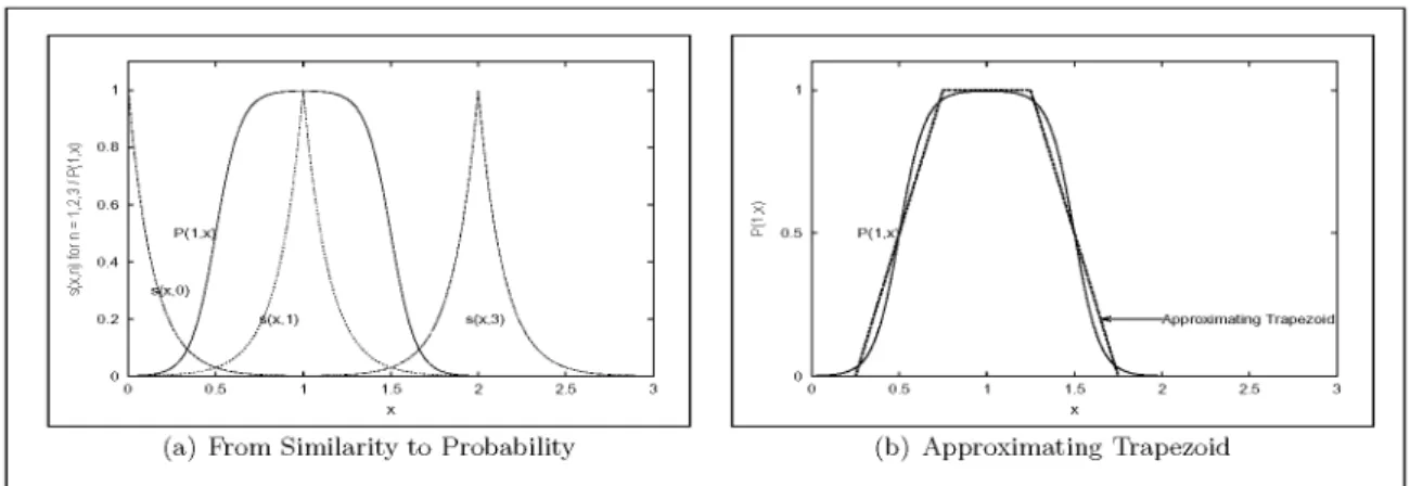
Now fix a finite setP = fp 2 Ng of points in the state space of a non-numeric linguistic vari-able. The probability that a state y 2 0 jPj], will be generalised to a 2 P can be found as follows.

The similarityη of any pointy to a fixed point a 2 P is given by η(a y) = e

;αd(a y). The probability that a pointy 2 0 p]is generalised toa2 pis given by

P(ajy)=

η(a y) Pp

n=1

η(n y)

(2) If η(k x) = 0 for k 2 P a;1 k a+1 withb =a;1 andc= a+1, then the proba-bility that a pointx 2b c]will generalise toa is given by

P(ajx)=

η(a x)

η(b x)+η(a x)+η(c x)

forx 2b c] (3)

For example if d(x y) = 1 and α = 7 then

η(x y) = e

;αd(x y)

0 as can be seen in Fig-ure 2.

Fig. 2.e;α

Define

η0

(x y)=

e;7d(x y)

d(x y)<1 0 d(x y)1:

(4) Then by(3)the probabilityPthat a pointy 2R generalises to the ordinal 1 is approximated by:

P(1jy)=

η0 (1 y)

η0

(0 y)+η 0

(1 y)+η 0

(2 y) fory 20 2]:

Theorem 7 can be applied by defining tolerances

ξ andζ such that 1ξaifP(1ja)0:95 and 1ζb if P(1jb) 0:05 then 1ξa if ja ;1j/0:25 and 1ζb if jb ;1j/0:75. Hence the set of neighborhoods fN(1) N

0

(1)g with N(1) 2 ξ andN0

(1) 2 ζ is a filter base and the distribu-tion can be approximated by a fuzzy set with

µ1(a) = 1 for a 2 10:25 and µ1(a) = 0 for a 2= 10:75 to give the trapezoidal fuzzy intervalh0:25 0:75 1:25 1:75ias illustrated in Figure 3. This process can be generalised to any i 2 N 0 i jLjso thatli is represented by the fuzzy intervalhi;0:75 i;0:25 i+0:25 i+ 0:75i

Linguistic terms modeled this way fulfill the as-sumptions in section 2.2. In the present section a fuzzy integer is denotedei.

Preorder

The set of fuzzy integers is pre-ordered with e0

<<enmirroring the natural order on the integers which is a chain.

Kernels

For eacheithere is a valuei

2 N to which only that term applies. Similarly for eachig

jthere is an intervali j] to which only that term ap-plies.

Pairwise tolerance

Adjacent fuzzy integersei g

i+1 are pairwise tol-erant sinceei

\ g i+16=.

Pairwise concatenation

The operation of joinon adjacent fuzzy inte-gers is defined pairwise to give fuzzy intervals. So that ea

g

a+i is represented by the fuzzy interval

ha;0:75 a;0:25 (a+i)+0:25 (a+i)+0:75i:

Support

The support of a fuzzy integer ea is given by supp(ea

)=a;0:75 a+0:75]and for a fuzzy intervalea

g

a+ibya;0:75 a+i+0:75].

Products

The product of two sets of fuzzy integers terms is defined on their product space to give the pair(ei1 ie2

)and naturally extended to Qp

1to

give(ie1 iep). The product space is partially ordered.

It has been shown that, given a reasonable set of assumptions about the structure of vague non-numeric linguistic variables, they can be mod-eled with fuzzy sets, filter bases or tolerance spaces. We have also shown an equivalence between these representations.

5.1. Modeling Numeric Linguistic Variables

The modeling of numeric linguistic variables is well established and they can be acquired using parametric method outlined by Kuz’min Kuz’min 1981]or outlined in any of the stan-dard textsKlir 1995, Zimmermann 1990]. The techniques outlined above can also be adapted and applied in a numeric context.

5.2. Weighted Linguistic Variables

In applications numeric representations of lin-guistic variables are usually normalised since there is no common measurement scale between variables Koczy 1993]; there is also often a measure of relative importance attached to dif-ferent linguistic variables. Relative importance can be handledEsbogue 1980, Esbogue 1983, Zimmermann 1990, Yager 1978] by applying a weighting to each variable, using extended scalar multiplication. The relative weight of variables can be obtained by techniques such as Saaty’s Saaty 1980] Analytic Hierarchy Pro-cess. It is possible to use this process to pro-duce fuzzy weightsLaarhoven 1983], however, in this paper only crisp weights will be used. The tolerance spaces used in this work are all bounded and normalised, in addition all weight-ings found by the AHP are in the inteval 0 1] hence applying a weighting is equivalent to applying a scaling factor to the whole space. Hence, w 20 1]can be applied to a tolerance space using a scaling()function

:0 1] h0 1] ξi!h0 w] wξi by:(w x)7!wx

this is equivalent to extended scalar multipli-cation Klir 1995] of a fuzzy number or fuzzy interval wheree

R denotes the set of trapezoidal fuzzy intervals.

:R e

R !

e R

:(w ex)=hwx1 wx2 wx3 wx4i

whereexis represented by the trapezoidal fuzzy sethx1 x2 x3 x4i.

6. Sparse Rule Bases

In decision support the aim is to associate an input casecmtaking a set of values(fli v

kg cm) which is an (intent, extent) pair (see section 6.1.)with a particulardjwith values(fli v

kg dj). If intent(fli v

kg cm) \ intent(fli v

kg dj) = intent(fli v

kg cm) then cm ! dj. If all possi-ble values taken by a variapossi-ble can be assigned to a decision type so that:

n

j=1 (fli v

kg dj)=(LV D) (5) and the same values are not taken by different decision types that is:

n \

j=1

intent(fli v

kg dj)= (6) the set valued function Dec : (LV D) ! D, Dec(fintent(li v

k dj)g) 7! dj is a bijection and the “rule base” is complete. If

n

j=1 (fli v

kg dj)6=(LV D)

and still 6 holds then Dec is not a bijection and the rule base is incomplete. The smaller the number of values for which exact partitions ex-ists the more sparse the rule base.

In the absence of a complete rule base Albrecht Albrecht 1998] suggests that uniform topolo-gies may be used to find partial or incomplete mappings between inputs and outputs of a rule base. Uniform topologies are a generalisation of metric spaces and generalise the notion of dis-tance between objects. A pre-ordered set has a uniform topologyPage 1978]and it is possible therefore to use generalised notions of distance within such sets.

6.1. Prototype Theory

Prototype theoryRosch 1988] seeks to model aspects of human cognition, according to Hamp-tonHampton 1993]the standard prototype mo-del

:::assumes that concepts are defined by a set of intensional [sic] proper-ties which determine the reference of the concept term to sets of objects in the world as extensions.

To make this clear, the extent consists of all objects belonging to a concept and the intent is the collection of attributes shared by the ob-jects. A prototype of one class is highly dis-similar to prototypes of another class Rosch 1988] and does not generally consist of a sin-gle exemplar. This aspect of prototype the-ory is particularly useful in structuring know-ledge acquisition where non numeric linguis-tic variables are used since it is reasonable to assume that if P1 and P2 are prototypes then

intent(P1)\intent(P2)= since thenP1 P2. It also suggests that in acquiring prototypes from experts a range of exemplars is required.

6.2. Structured Knowledge Acquisition in Vague Environments

In this section we introduce an algorithm for structured knowledge acquisition, the following are definitions required both here and in section 9.

Definition 23. (Maximum (Minimum) Term)

A maximum (minimum) term is the greatest (least) point of a concatenated linguistic term. A maximum (minimum) term represented by a trapezoidal fuzzy interval is amaximum( mini-mum)point.

Definition 24. (Anchor Term) An anchor term is the most representative point of a con-catenated linguistic term, in general it is the minimum (maximum) member of a concate-nated term which includes the least (greatest) member of the whole term set. Otherwise it is the central term(s). An anchor term rep-resented by a trapezoidal fuzzy interval is an anchor point. The anchor point is analogous to Zeleny’s [Zeleny 1991] notion of an ideal point in multi criteria decision making.

The algorithm is as follows:

1. Acquire a set of decision typesD(see section 2.2.) from user

2. Acquire a set of linguistic variablesVwhich are used to distinguish decision types from user.

3. Associate eachv_kwith one or moredjto give the pairs(vk dj).

4. Acquire prototypical minimum and maxi-mum values for (li v

k dj) from l0v

k ::: ln v

k

and form the meet as the concatenated term (lmin maxv

k dj) select an anchor term which must be present(usually the max or min of the term set).

The following example based on one that ap-pears inWolkenhauer 1999]illustrates this pro-cess.

Example 16. (Applying the Algorithm) Sup-pose we have a decision about whether to pass or fail a student following an assessment. Then D= fpass, failg. For the purposes of illustra-tion, suppose there are two linguistic variables V =fmark, seminargbecause where a student is borderline the exam board considers evidence about their seminar performance (seminar) in reaching a decision. Each variable is associ-ated with a decision to give the pairs (mark, pass), (seminar, pass), (mark, fail)and (sem-inar, fail). The union of pairs with the same extent that isj(vk ej)gives(variable decision) pairs, for example(fmark, seminarg fail). The pass mark is 40 but it is known that this may reflect a mark in the range35 45] because of marker variability, representing marks as trian-gular fuzzy sets using the theory linking toler-ance spaces and fuzzy sets, thepass markg is a fuzzy seth35 40 45iand any markmis repre-sented by the fuzzy numberme =hm;5 m m+ 5i. The variableseminartakes values from the pre-ordered set

performance=fnone, very poor, poor,

mediocre, competent, excellent, superbg:

can handle at any time Miller 1956] and that used in comparable fuzzy systemsGodo 1989]. The prototypical minimum and maximum val-ues for (performanceseminar pass) are f

com-petent, superbgand the concatenated term set isfcompetent excellent superbg. The proto-typical term set for(performanceseminar fail) is fnone, very poor, poorg. For the numeric linguistic variable a similar process gives (emmark pass

) = e

40 so (emmark fail ) =

e 35. The rule base is sparse because pairs such as (

e

35mark excellentseminar)do not have a known extent and are not included within the know-ledge base of cases which have a known deci-sion type.

7. Reasoning in Sparse Rule Bases

In the absence of a complete rule base some other means of inference is required. The ap-proach taken here takes Hume’s view that:

All kinds of reasoning consist in noth-ing but a comparison, and a disco-very of those relations, either con-stant or inconcon-stant, which two or more objects bear to each other.

(D.Hume,The Treatise, Book I, Part III, Section II)

Suppose for a given inference we have a body of evidenceE and a hypothesisHbut no prob-abilistic data, function or relation mappingE to H. In the decision making context this is equiv-alent to having a known decisiondj and a case to be classifiedcjand no firm data linkingdjto cj. Then, one way forward is to use similarity or possibility-based methods.

RuspiniRuspini 1996]characterizes possibilis-tic reasoning as follows:

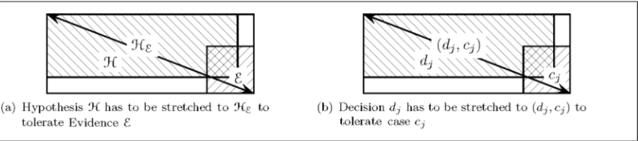
Possibilistic reasoning methods, :::, determine if there is a modified ver-sion ofH(or relaxation) that is con-sistent with the evidence E. We may say that we are trying tofind out how far we need to stretch or relax] the truth tofit the hypothesis to the evi-dence. Possibilistic methods exploit relations of similarity and of rela-tive preference between alternarela-tive explanations of the evidence.

Figures 4 and 5 illustrate this process and show how it may be applied to decision making. Similarity is reflexive and symmetric but not transitive and the process can therefore also be seen as determining how far a hypothesis must be stretched(relaxed)to tolerate the evidence.

Fig. 4.Possibilistic Reasoning — stretching the hypothesis to tolerate the evidence.

This notion of stretching or relaxing a hypoth-esis is closely related to the idea of transfor-mational distance proposed by both Hahn and Chater Hahn 1997] and Imai Imai 1977] in the cognitive literature. The tolerances used in section 3. are an example of this kind of stretch-ing. The tolerance can be seen as the maximum amount a hypothesis about the application of a linguistic variable can be stretched and still hold. SoN(1)retains a degree of“oneness”on all of(0 2)but not at 2 and 0.

8. Distances between Vague Points

In section 4. we showed that linguistic terms could be modeled with fuzzy numbers, toler-ance spaces, and filter bases and that these rep-resentations are homomorphic. This gives three possible approaches to finding the distance be-tween vague points. Before doing so, we firstly introduce some distance measures which may be useful in developing the arguments.

8.1. Metrics, Pseudo-metrics, Separations andT0-metrics

Definition 25. (Metrics and Pseudo-metrics)

Ametricis a function d:X X !R such that the following conditions hold:

M1 d(x y)0 d(x y)=0,x =y

M2 d(x y)=d(y x);8x y 2X.

M3 d(x y)+d(y z)d(x z)8x y z2X. Apseudo-metricis a function dp :X X !R such thatM1is replaced by:

PM1 dp(x x)=0.

These definitions produce the well known Haus-dorff orT2spaces. A function can also be

spe-cified to find the separation between intervals as follows:

Definition 26. The Hausdorff separation is a non-symmetric function [Diamond 1994] (Fi-gure 6) on two sets given by:

S ds

H(A B)=supfd(a B):a2Ag.

This function is not a metric since d_Hs(A B)=0 but A6=B is possible.

Fig. 6.Hausdorff separation ofAandB.

The Hausdorff distance is a metric [Diamond 1994] on the sets A and B given by dH(A B)= maxfd

s

H(A B) d s

H(B A)g

Whilst the Hausdorff separationSshows how to construct a non symmetric distance measure a T0metric(definition 27)shows how minimality may also be dispensed with.

Definition 27. (T0-Metric)A T0metric[O’Niel

1998] is a set X, with a function t:X X!R such that the following axioms hold:

T1 t(x x)=t(x y)=t(y y))x =y.

T2 t(x y)t(x z)+t(z y);t(z z)

8x y z2X.

A space with this set of axioms has aT0

topo-logy as follows.

Definition 28. Let (S t) be a space equipped with a T0metric. Then for x 2S and0<ε 2R define anopen ball

B_ε(x)=fy2S: t(x y)<t(x x)+εg

Lemma 1. If(S t)is a space equipped with a T0 metric then the open balls of S are a basis

for a T0topology on S.

Proof. Suppose thatB_εx(x) andBεy(y) 2 (S t) and thatz 2Bε

x(x)\Bε

y(y), next define

δ =min(t(x x)+εx;t(x z) t(y y) +εy;t(y z))>0 now show thatB_δ(z)Bε

x(x)\Bε

y(y). Supposez0

2Bδ(z)then byT2 t(x z

0

)t(x x)+t(z z 0

);t(z z)

and z0 2 Bε

x(x). It can be shown in a similar way thatz0

2Bεy(y). SinceS= x 2SB1

(x)the open balls form a basis for a topology onS. Suppose x y 2 S and t(x x) < t(x y); let

ε = t(x y);t(x x) > 0 then x 2 Bε

x(x) but y 2= Bε

x(x). Hence the topology of (S t) is T0.

Note that T1establishes identity, but does not require symmetry or minimality. T2 is the tri-angle inequality modified to allow non zero self distances.

Example 17. All metrics are trivially T0

met-rics since d(x x) = d(x y) = d(y y) = 0 im-plies x = y and d(x y) d(x z)+d(z y); d(z z)since d(z z)=0.

Example 18. As a more substantive example, let X be the set of closed intervals a b] 2 R then

t :X X !R

t(a1 b1] a2 b2])=maxb1 b2];mina1 a2] is a T0metric but not a metric [Matthews 1997].

In section 3.1. it was established that the topo-logy of a vague set of linguistic terms wasT0,

but not necessarily T2 the use of a T0 metric

reflects this fact. TheT0metricin example 18

can be applied to the separation of a pointpand intervalI =a b]so that

D(p I)=max(t(p a) t(p b));t(I I) which gives

D(p I)

>0 p62I 0 p2I

a property which will be useful in section 9.

8.2. Distance Measures and Cognitive Similarity

The metric basis for similarity is proposed by Shepard in theUniversal law of Generalisation:

A psychological space is established for any set of stimuli by determining metric distances between the stimuli

such that the probability that a re-sponse level to any stimulus will gen-eralise to any other is an invariant monotonic function of the distance between them.

TverskyTversky 1997]on the other hand raises two major objections to the metric basis of sim-ilarity.

Minimality – M2, PM1is questioned because the probability of judging two stimuli as dif-ferent is not constant for all stimuli. In recognition experiments an object may be identified with another object more often than it is with itself.

Symmetry – M2 is questioned because many statements of similarity appear to be direc-tional soais likebrather thanbis likea. For instance, an ellipse is judged more similar to a circle than a circle to an ellipse. Note that this is an asymmetry in the judged degree of similarity, not a denial of the reflexivity of similarity.

These objections can be overcome fairly straight-forwardly when generalizing the metric space axioms to apply to intervals rather than points: the minimality objection by having a mapping into R (as in a T0 metric) instead of R

+ the symmetry objection by using non-symmetrical directional separation functions reflecting the fact that a hypothesis must be stretched or re-laxed from some fixed point beyond which it no longer holds.

If a metric-based approach is accepted, the ques-tion then arises of what specific metric best models the intuitive approach which people have. Attneave Attneave 1950] and Shepard Shepard 1980]both suggest thed1orcity block metric given by equation 7

d1(xi yi)= n X

i=1

jxi;yij (7) is the most appropriate. Shepard makes the par-ticular point that

The isometric curves for the city block metric are continuous but not differentiable. The com-pression of an axis by weighting can therefore mean minor shifts in adjudged distance cause major shifts in judged similarityEveritt 1997]. In section 9. a distance measure is defined which whilst a metric for points is not for intervals. This measure also meets Tversky’s objections. Summation will be applied in a way which gives a d1 metric when it is applied to

multi-dimensional points.

8.3. Fuzzy Approaches

There are number of approaches to finding the distance between fuzzy sets in the literature Klir 1995, Diamond 1994, Goetschel 1993, Koczy 1993, Kaleva1987]. Most are based on the Hausdorff distance between the alpha-level cuts or the extension principle. However these approaches are not guaranteed to produce output sets of the same nature as the input sets Dia-mond 1984, Hsiao 1996]. In empirical studies it has been found that the similarity measures on fuzzy sets which correlate best with the similar-ity between the verbal descriptions of those sets are those which are based on the kernels(

e A1), or the centre of gravity of the fuzzy setsYoshikava 1996, Zwick1988]. These are important find-ings which lend further weight to the tolerance space model of fuzzy sets discussed earlier. Another approach to fuzzy numbers is to treat them as tolerance spaces. We have already shown in section 4. how we can derive fuzzy sets from a tolerance space. Distances in a toler-ance space can be treated as tolertoler-ance mappings (definition 13)for example

d:hR ξi hR ξi!hR ξi d(x y)=jx;yj

This is easily translated to a fuzzy set using the techniques outlined earlier.

9. Distances between Cases and Prototypes

In this section, a proposal for a distance mea-sure, which meets the criteria outlined for it in the preceding sections, will be made. Since

prototypes are composed of concatenations of linguistic terms, they are represented by inter-vals rather than points. The notion of an anchor point introduced in section 6.2. will be needed again here. The considerations discussed in sec-tions 4. and 7. will also be taken into account.

Example 19. The anchor term offcompetent excellentsuperbgtaken from the pre-ordered set

performance=fnone, very poor, poor,

mediocre, competent, excellent, superbg

is superb. The anchor term of fpoor

medi-ocrecompetentgismediocre. In applications these terms are represented by a fuzzy number which may be referred to as theanchor point. The distance between two terms described by fuzzy numbers can be found as follows. Let

e

A = ha1 a2 a3 a4ithen its centre is c( e A1) is (a2+a3)=2 and the alpha-cut at 1 gives a toler-anceτ(

e

A1)= (a3;c)the alpha-cut at 0 gives the tolerancesτL(

e

A0) = c;a1 and τR( e A0) = a4;cso

e

A=hc;τL c;τ c+τ c+τRialso denotedhc;(τ τL τR)i.

For the prototype(intent, extent)pair

P=( k Y

i=1 WiPe

i P)

and the case pair

C=( k Y

i=1 WiCe

i C)

where Wi is the weight for theith variable the weighted distance between the centres of the intent termsc(D)is:

c(D) : e R n

e R n

!R

c(D(C P))= n X

i Wi

8 > > <

> > :

c(Ci);c(max(Pi)) ifc(anchor(Pi))c(Ci) c(min(Pi));c(Ci) ifc(anchor(Pi))>c(Ci)

(8) where e

R n

is the set of trapezoidal fuzzy sets hx1 x2 x3 x4idefined onR

Then the expression for the distance between case and prototype becomes

D: e R n

e R n

! e R n

D(C P)=

c(D);(maxfWiτig maxfWiτi

Lg maxfWiτi

Rg))

which is the trapezoidal fuzzy interval

c(D);maxfWiτi

Lg c(D);maxfWiτg c(D)+maxfWiτg c(D)+maxfWiτi

Rg

:

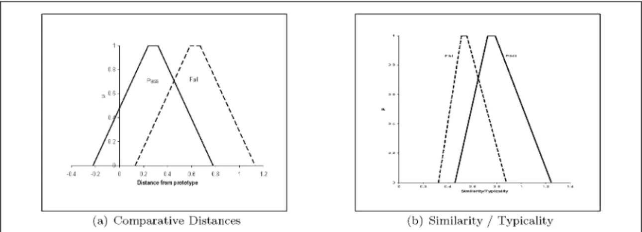
Similarity can then be calculated as a function of distance as in section 7. Similarity measures based on D meet all of Tversky’s objections to distance based similarity. D does not imply minimality, since a case may be closer to a pro-totype than to itself as self distance is around 0 but distance from a prototype may be negative. A negative distance implies that, rather than be-ing similar to the prototype, the case is to some extent atypicalexample of that prototype Os-herson 1997], unlike similarity which is usually expressed in the interval0, 1] typicality is not necessarily bounded aboveOsherson 1997, pp 190]. In decision making this is the type of case whose outcome is immediately obvious to a hu-man decision maker. In the student domain this could be a student with a mark in excess of say 80 whose performance is excellent; such a stu-dent is typical of the kind of stustu-dent we would wish to pass, and more typical than a student with a mark of 45 who has performed compe-tently in seminars. However both are examples of the pass prototype.

The measured extent of similarity/typicallity based onDis also neither symmetric nor transi-tive. However, when applied to the crisp num-bers, D is the d1 (city block) metric, as sug-gested in section 3.1., and symmetry and tran-sitivity are restored.

Example 20. Having acquired prototypes in example 16, the student example is developed further. Suppose that student obtains a mark of 38 and their performance in seminars is excel-lent. Should that student be passed or failed? Marks have been found to be 10 times more important than seminar performance in making this decision.

The fail prototype is represented by the(intent, extent)pair

Pfail=(hfnone, very poor,poorg 0 35]i

fail)

the anchor terms arenoneand 0; the maximum terms arepoorand 35. This gives the following giving the numerical representation:

Pfail =

h0 3];h0:25 ;0:75 +0:75ii h0 35] h0 5 5ii fail

with the centres of the anchor and maximum points given by

c(anchor(0 3]))=0,c(anchor(0 35]))=0; and

c(max(0 3]))=3,c(max(0 35]))=35 which is normalised to

Pfail

h0 0:5] h0:04 ;0:13 +0:13ii h0 0:35] h0 ;0:05 +0:05ii fail

Similarly the pass prototype is represented by the(intent, extent)pair

Ppass =

hfcompetent, excellent,superbg

40 100]i pass

giving the normalised numerical representation of the pass prototype as

Ppass

h0:75 1] h0:04 ;0:13 +0:13ii h0:4 1] h0 ;0:05 +0:05ii pass

applying the weighting to the mark variable gives

Pfail

h0 0:5] h0:04 ;0:13 +0:13ii h0 3:5] h0 ;5 +5ii fail

and

Ppass

h0:75 1] h0:04 ;0:13 +0:13ii h4 10] h0 :5 +5ii pass

a similar exercise for the input case

C=(hexcellent 38i case) gives

h0:83 h0:04 ;0:13 +0:13ii h3:5 h0 ;5 +5ii case

Applying equations 8 and 9 gives

D(C Pfail)=h0:13 0:59 0:67 1:13i and

D(C Ppass)=h;0:22 0:24 0:32 0:78i Similarity(η) can be calculated by applying a continuous monotone function; an exponential functionη =e

;Dis used here.

η(C Pfail)=h0:32 0:51 0:55 0:88i and

η(C Ppass)=h0:46 0:73 0:79 1:25i

10. Outputs and Outcomes

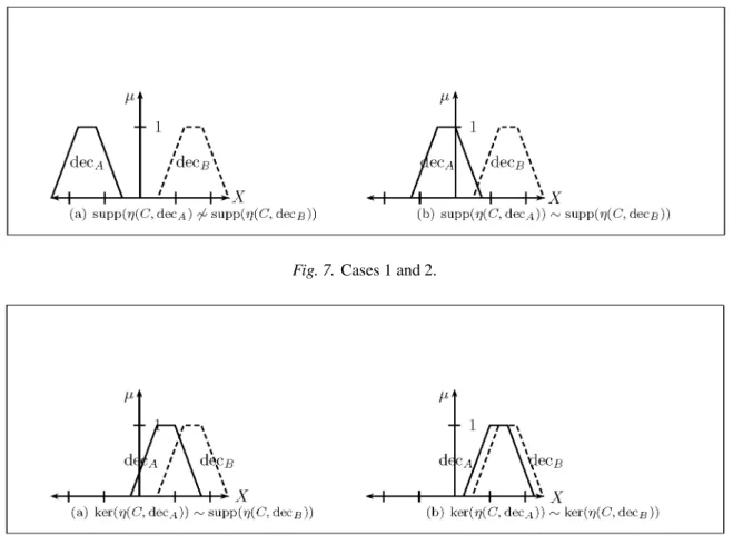
There are five possible outcomes, four of which are illustrated in Figures 7 and 8.

In these figures decA is the set representing

η(C decA) (the similarity of an input case to

decision prototype A) and decB the set repre-senting η(C decB) where decX is a decision prototype and C is a case. The support and the kernel of the fuzzy set are denoted supp and ker respectively and it is assumed in cases 1 – 4 that ker(η(C decA))- ker(η(C decB))

Case 1supp(η(C decA))6 (η(C decB)), Fig-ure 7(a). Where decision prototype decB is strongly preferred. A person would not usually hesitate to make this decision and might describe it as self evident.

Case 2supp(η(C decA))supp(η(C decB)), Figure 7(b). Where decision prototype decBis preferred. A person would usually make this decision and without difficulty but it would not be self evident.

Case 3 ker(η(C decA)) supp(η(C decB)), Figure 8(a). Where decision prototype decBis weakly preferred. A person would perhaps be hesitant in making this deci-sion but would usually be content to make it on the basis of the evidence.

Fig. 7.Cases 1 and 2.

Case 4 ker(η(C decA)) ker(η(C decB)), Figure 8(b). Where decision prototype decBis very weakly preferred. These are the cases where a person would usually consider it advisable to apply another test (assuming one is available) before mak-ing a decision.

Case 5ker(η(C decA))=ker(η(C decB)). Where it is undecidable which decision prototype decAor decBis preferred. These are the cases where a person would want to apply another other test(or flip a coin!) before making a decision.

This process allows a mapping from linguistic inputs to linguistic outputs.

Example 21. Returning again to the exam-ples 16 and 20 we have the output sets shown in Figure 9 which shows supp(η(C Pfail)) ker(η(C Ppass))So a decision to pass is weakly preferred. This reflects the kind of decision that might be made in reality given these cir-cumstances. A student with a mark of 38, but an excellent seminar record, would usually be passed – but only just. For this example we could have the following pre-ordered set of lin-guistic outputs

poor fail - fail - just fail - viva voce

-just pass - pass - good pass.

Case 4 and case 5 have been assigned the same linguistic output on this scale.

If the two distances do not overlap, then the course of action should be clear. If they do overlap, then it may be that an alternative way of distinguishing between the alternatives should

be considered depending on the degree of un-certainty. In this domain it indicates if there is a case for giving the student aviva voce; in other domains it might trigger the use of some other additional selection test. A measure of the degree of overlap is given by intersection of the membership functions. So in this exam-ple the case for giving the student aviva voce is stronger than the case for not doing so since

µD(C PFail)

(x)\µD

(C PPass)

(x)0:7. This gives a decision maker an alternative way of resolving the case should they wish to do so.

11. Conclusion

By starting with an intuitive set of assumptions about the mathematical properties of a set of non numeric linguistic terms it has been shown that pre-ordered sets of linguistic terms can be modeled with fuzzy numbers, filter bases and tolerance spaces. Using filter bases and toler-ance spaces allows the disttoler-ance between fuzzy numbers to be found in a way which is consid-ered more intuitive than the usual approaches based on the extension principle for fuzzy num-bers. The use of a measure which is not a met-ric to find distances between cases and proto-types overcomes objectionsTversky 1977] to a purely geometric approach to similarity. The relative distance of input cases from different decision prototypes gives fuzzy numbers which can then be used for similarity-based reasoning in sparse, linguistically valued rule bases. The relative positions of the output fuzzy sets also make it possible to devise pre-ordered sets of