Miller_unc_0153D_19334.pdf

DARK MATTER AND DARK ENERGY IN THE EARLY UNIVERSE

Carisa A. Miller

A dissertation submitted to the faculty of the University of North Carolina at Chapel Hill in

partial fulfillment of the requirements for the degree of Doctor of Philosophy in the

Department of Physics and Astronomy.

Chapel Hill

2020

Approved by:

Adrienne Erickcek

Jon Engel

ABSTRACT

Carisa A. Miller: Dark Matter and Dark Energy in the Early Universe

(Under the direction of Adrienne Erickcek)

TABLE OF CONTENTS

LIST OF FIGURES . . . .

vi

LIST OF ABBREVIATIONS AND SYMBOLS . . . viii

1

Introduction . . . .

1

2

Dark Energy:

Quartic Chameleons . . . 10

2.1

Classical Chameleons

. . . 12

2.1.1

Chameleon Cosmology . . . 14

2.1.2

Quartic Chameleons . . . 16

2.2

Quantum Chameleons . . . 19

2.2.1

Particle Production . . . 20

2.2.2

Effects of Particle Production for

κ

.

O

(1)

. . . 25

2.3

Kicking the Quartic Chameleon . . . 29

2.4

Discussion . . . 32

3

Dark Matter:

Impact of Nonthermal Production on the Matter Power Spectrum . . . 35

3.1

Nonthermal Production of Dark Matter . . . 36

3.1.1

Dark Matter Abundance . . . 36

3.1.2

The Adiabatic Cooling of Dark Matter . . . 41

3.2

Dark Matter Distribution Function . . . 43

3.3

Lyman-Alpha and MW Satellite Constraints . . . 47

3.3.1

Free-Streaming Length . . . 48

3.3.2

Transfer Function . . . 51

3.4

Discussion . . . 58

4

Interacting Dark Matter:

Impact of Nonthermal Production on the Matter Power Spectrum . . . 61

4.1

Interacting Nonthermal Dark Matter . . . 61

4.2

Dark Matter Distribution Function . . . 70

4.3

Free-Streaming Lengths . . . 72

4.4

Transfer Functions . . . 74

4.5

Discussion . . . 76

5

Conclusion . . . 79

LIST OF FIGURES

1.1

Chameleon effective potential in the exponential and quartic models . . . .

5

2.1

Evolution of the Chameleon Field and its Kinetic and Potential Energies . . . 18

2.2

Physical Wavenumber and Energy Density in Perturbations . . . 24

2.3

Decay of Chameleon Energy Due to Redshifting and Particle Production . . . 31

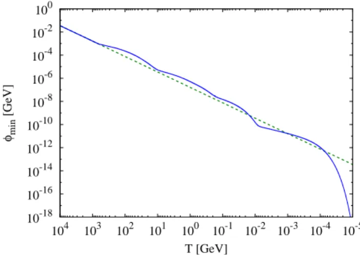
2.4

Evolution of

φ

. . . 33

2.5

Response-time of the Chameleon Field . . . 34

3.1

Energy Density Evolution of a Pressureless Fluid, Radiation, and Dark Matter . . . 37

3.2

Evolution of the Average Dark Matter Velocity During an EMDE . . . 42

3.3

“Birth Time” Distribution Function for Nonthermal Dark Matter Production . . . 45

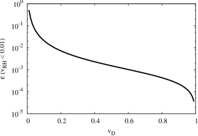
3.4

Fraction of Dark Matter that is Nonrelativistic at Reheating as a Function of

v

. . . 45

3.5

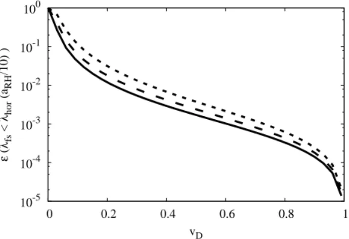
Fraction of Dark Matter Cold Enough to Preserve EMDE-Enhanced Structure

Growth as a Function of

v

. . . 46

3.6

Fraction of Dark Matter Cold Enough to Preserve EMDE-Enhanced Structure

Growth as a Function of

T

. . . 47

3.7

Dark Matter Free-Streaming Length as a Function of

γ

. . . 50

3.8

Comoving Momentum Distribution Function for Nonthermal Dark Matter . . . 52

3.9

Nonthermal Dark Matter Transfer Functions . . . 53

3.10 Nonthermal and WDM Transfer Functions with Matched Half-Mode Scales . . . 54

3.11 Fits for the Parameters

β

and

γ

as a Function of

ln(α)

. . . 54

3.12 Limits on

γ

and

T

. . . 56

3.13 Relationship Between the Fitting Parameter

α

and the Free-streaming Length . . . 57

4.1

Evolution of

γv

with Scale Factor for Several Values of

σ

˜

. . . 64

4.2

Evolution of

γv

with Scale Factor with Analytic Estimates of Late-Time Behavior. . . 66

4.3

p(10a

)

and a Function of

a

for Several Values of

σ

˜

. . . 67

4.5

Evolution of

γv

with Scale Factor for Select Values of

σ

˜

and Several Values of

a

. . . 69

4.6

Comoving Momentum Distribution Functions for Interacting Nonthermal Dark Matter . . . 71

4.7

Interacting Nonthermal Dark Matter Transfer Function . . . 74

4.8

Interacting Nonthermal Dark Matter Transfer Function . . . 75

4.9

Interacting Nonthermal and WDM Transfer Functions with Matched Half-Mode Scales . . . 76

LIST OF ABBREVIATIONS AND SYMBOLS

a

Scale factor

˜

a

Jordan frame scale factor

a∗

Einstein frame scale factor

a

Scale factor today

a

Scale factor at a dark matter particle’s production

a

Scale factor at time

t

a

Scale factor at reheating

b

Number of dark matter particle produced per scalar decay

BBN

Big Bang Nucleosynthesis

c

Speed of Light

CDM

Cold Dark Matter

C.L.

Confidence Level

h

E

i

Average energy per dark matter particle

EFT

Effective Field Theory

EMDE

Early Matter-Dominated Era

F

(x

, x

)

Elliptic integral of the first kind

f

Fraction of scalar field energy transferred to dark matter

f

(x)

Distribution function of variable

x

G

Gravitational constant

g∗

Chapter 2: Determinant of the metric

g

g∗(T

)

Number of relativistic degrees of freedom at temperature

T

g∗

(T)

Number of relativistic degrees of freedom in the entropy density at temperature

T

g

Metric that solve the Einstein equations

˜

g

Metric that governs geodesic motion

H

Hubble Parameter

H∗

Einstein frame Hubble Parameter

h

Hubble fudge factor:

H(a

) = 100h

km/s/Mpc

K

Kinetic energy of the chameleon field

k

Chapter 2: Comoving wavenumber of a chameleon field plane-wave perturbation

k

Chapter 3&4: Comoving wavenumber of a perturbation mode with length

λ

k

Boltzmann constant

k

Comoving free-streaming wavenumber (with

a

= 1

today)

k

Half-mode scale

k

Physical wavenumber of a chameleon field plane-wave perturbation

M

Mass scale of a chameleon runaway potential

M

Solar mass

m

Mass

MCMC

Markov Chain Monte Carlo

M

Half-mode mass

M

Planck mass

MW

Milky Way

m

Dark matter mass

n

An integer

nCDM

nonCold Dark Matter

N

Effective number of neutrinos

n

Occupation number

ˆ

n

Comoving number density of

φ

particles

ˆ

n

Comoving number density of dark matter particles

P

Pressure

P∗

Einstein frame pressure

P

(k)

Matter Power Spectrum

p

Chapter 2:

p

≡

ln(a∗/a∗

)

p

Chapter 3&4: Momentum

p

Dark matter particle momentum long after kinetic decoupling

p

“Floor” of the dark matter momentum

P

Matter Power Spectrum in a scenario with non-cold dark matter

q

Comoving momentum scaled by the comoving momentum of a typical dark matter particle

QCD

Quantum Chromodynamics

R∗

Ricci Scalar

SM

Standard Model

T

Radiation temperature

t

Proper time

T

Temperature at matter-radiation equality

t

Initial proper time

T

Jordan frame radiation temperature

T

Kinetic decoupling temperature

T

Reheat temperature

T

Stress Energy Tensor in the Einstein frame

˜

T

Stress Energy Tensor in the Jordan frame

T

Neutrino temperature

T

Dark matter temperature

T

(k)

Transfer function

V

(φ)

Potential of the chameleon field

v

Velocity

v

Velocity imparted to a dark matter particle at its production

V

Effective potential

w

Equation of state parameter

WDM

Warm Dark Matter

w

Dark matter equation of state parameter

X

γ

v

Y

(γ

v

a

)

z

Redshift

α

Fitting parameter for the dark matter transfer function

β

Chapter 3&4: Fitting parameter for the dark matter transfer function

Γ

Scalar field decay rate

γ

Fitting parameter for the dark matter transfer function

γ

Lorentz factor

γ

Lorentz factor of velocity

v

δφ

Perturbation to the chameleon field

ε

Fraction of dark matter particles

κ

Chameleon self-interaction constant

λ

Comoving wavelength

Λ

CDM

Λ

Cold Dark Matter

λ

Comoving free-streaming length

λ

Physical free-streaming length today

λ

Horizon size

µ

γ

v

a

/a

π

Delicious

ρ

Energy density

˜

ρ

Jordan frame energy density

ρ∗

Einstein frame energy density

ρ

Critical energy density

ρ

Energy density in perturbations

ρ

Radiation energy density

ρ

Scalar field energy density (chameleon or otherwise)

ρ

Dark matter energy density

Σ

Chapter 2: The kick function

Σ

Chapter 4: Momentum transfer rate

σ

Initial momentum transfer rate

h

σ

v

i

Dark matter velocity-averaged annihilation cross section

φ

Scalar field (chameleon or otherwise)

ϕ

Dimensionless chameleon field:

φ/M

χ

Dark matter particle

Ω

Fraction of the critical density in dark matter

CHAPTER 1

Introduction

Two of the most pursued questions in cosmology are the nature and composition of what we appropriately

call dark energy and dark matter. Dark energy is the term for the force that drives the current accelerated

expansion of the Universe and makes up

68.89

±

0.56%

(68% C.L.) of the total energy density today [1]. Dark

matter accounts for a remaining

26.07

±

0.53%

[1] and thus far has only been detected only by its gravitational

interactions. The first definitive evidence that our Universe was not only expanding, but expanding at an

accelerated rate, was provided by observations of Type Ia supernovae [2, 3]. More recently, observations

of baryon acoustic oscillations and clustering in large scale structure provide another measurement of the

current expansion rate [4]. The original evidence for dark matter came from the discrepancies in observations

of dynamical and luminous mass of galaxies and clusters; the mass inferred from observed motion was much

larger than the mass accounted for by luminous objects. The use of the term “dark matter” is attributed to

Fritz Zwicky who estimated the mass of the Coma cluster using the radial velocity of galaxies within the

cluster, and found it to be much larger than the mass inferred from the number and brightness of the galaxies,

leading him to conclude the presence of additional, nonluminous matter [5]. Further evidence came when

Vera Rubin and collaborators used spectrography to measure, in M31, the radial velocities of stars and gas at

varying distance from the galactic center and found a flat rotation curve implying the presence of additional

mass [6]. The presence of dark matter has also been inferred by using gravitational lensing to obtain the mass

of clusters, rather than dynamical motion [7]. Dark matter is also necessary to explain the observed structure

growth from measurements of anisotropies in the Cosmic Microwave Background (CMB) [8, 9].

In order to explain the Universe’s current phase of accelerated expansion using general relativity, one

must consider an additional energy component having a negative pressure so that its energy density remains

nearly constant as the Universe expands. Conforming with other cosmological observations, however, requires

this constant value of the energy density to be extremely small,

ρ

= 2.5

×

10

GeV

∼

10

M

(in natural units, where

M

is the Planck mass)[1]. While QFT predicts the existence of a vacuum energy,

Alternatively, one can introduce new physics by introducing a new scalar field or by modifying general

relativity. Popular modifications to gravity often take the form of

f

(R)

-theories in which the Einstein-Hilbert

action becomes a general function of the Ricci scalar

R

[10, 11, 12], and/or scalar-tensor theories in which

there is an additional scalar field which couples non-minimally to the curvature [13]. The simple inclusion of

an uncoupled scalar field can also give rise to cosmic acceleration if the field is presently confined to a near

constant energy value,

e

.

g

.

by evolving along a flat region of its potential [14].

Beyond being nonluminous, evidence of dark matter further indicates that it is a type of matter entirely

apart from baryons and leptons. Prior to recombination, baryons

and photons remain in a tightly coupled

plasma. This plasma will initially infall into overdense regions in the early Universe, but as the density

increases, radiation pressure builds until the plasma is forced outward. After the plasma is ejected from the

overdense region, the radiation pressure decreases, and the infall begins again. This oscillatory motion is

imprinted in the anisotropies of the Cosmic Microwave Background(CMB). In contract, dark matter does not

interact with baryons or photons, and continues to accumulate in overdense regions. From the comparative

amplitude of the first infall and first rebound, the contribution of both baryonic and nonbaryonic matter to

the total energy density can be calculated. It is from this that we know that

4.90

±

0.09%

of the energy

density in our Universe is baryonic matter, while another

26.07

±

0.53%

is nonbaryonic, dark matter [1].

Further confirmation of such a small fraction of ordinary baryonic matter comes from the abundances of light

elements predicted by Big Bang Nucleosynthesis (BBN) [15, 16]. The CMB also eliminates neutrinos as a

significant component of the dark matter, as neutrinos are relativistic at the time of recombination and are

able to freely stream from overdense regions. Thus, we are again required to look to new physics beyond the

SM in order to adequately explain cosmological observations.

The variety of theories and models invoked to explain dark matter and dark energy is extensive, and in

this work we present our explorations of single, well-motivated scenarios within each subject. The nature

of dark matter and dark energy are both highly pursued questions, and thus far investigations into each

have communicated the clear need for new, undiscovered physics, likely at energy scales not yet probed

by experiments. Such energy scales are reached in the high temperatures of the early Universe, and our

explorations use this period as a theoretical laboratory to study dark matter and dark energy.

1_{Throughout this work we will define baryons to include not only protons and neutrons, but electrons as well, despite the fact that}

To start these explorations we first lay down the basic cosmological framework that we will be considering.

A Universe that is homogeneous, isotropic, and expanding can be most generally described by the

Friedmann-Lemaˆıtre-Robertson-Walker space-time metric:

ds

=

−

dt

+

a

(t)dx

.

(1.1)

The expansion is characterized by

a(t)

, a dimensionless scale factor that increases with time,

t

. If we consider

two stationary objects in an expanding cosmology as two fixed points on an expanding grid, the distance

between the two can be described by the differences in their coordinates, which is fixed, or by the measured

distance between them, which increases as the grid size increases. We refer to these distances as the comoving

and physical distances, respectively, and they can be related at a given time by

d

=

a(t)d

. Clearly,

the comoving and physical distance are equal when the scale factor equals 1, and, while it is standard to

define today,

t

, as the point at which

a

=

a(t

) = 1

, it is an arbitrary choice and we will often choose to set

a

= 1

at another time through out this work. The rate at which the scale factor changes with time is known as

the Hubble rate:

H(t)

≡

da/dt

a

=

˙

a

a

(1.2)

If we assume the energy content of the Universe can be described by a perfect fluid which energy density

ρ

and pressure

P

, then, in a flat space-time, the Einstein field equations give us the first and second Friedmann

equations, which govern cosmological dynamics:

H

=

8πG

3

ρ,

(1.3)

¨

a

a

=

−

4πG

3

(ρ

+ 3P

).

(1.4)

Using the above equations one can derive the equation for energy conservation for a perfect fluid in an

expanding Universe:

dρ

which can be rewritten using the equation of state parameter,

w

≡

P/ρ

, as

ρ

=

ρ(t

)a

.

(1.6)

Thus we can see that for matter and other pressureless (

w

= 0

) fluids, their energy density decreases with time

according to

ρ

∝

a

, and we say the energy density “redshifts away” as

a

. For radiation, the equation of

state parameter is

w

= 1/3

and so

ρ

∝

a

.

If a substance has a negative pressure and an equation of state

w <

−

1/3

, then, according to the second

Friedmann equation (Eq. 1.4),

¨

a

is positive and the expansion rate is accelerating if this substance is the

dominant energy competent of the Universe. If the equation of state is

w

=

−

1

then

ρ

is constant and the

energy density of such a substance is not diluted by the expansion of the Universe. Current observations

provide bounds on the present value of the dark energy equation of state parameter:

w

=

−

1.03

±

0.03

[1, 17].

One such substance that could exhibit this behavior is a scalar field dominated by its potential energy. The

total energy density of a scalar field,

φ

, is given by the sum of its kinetic and potential energies

ρ

=

K

+

V

,

whereas its pressure can be given by

P

=

K

−

V

, and the equation of state for a potential-dominated field

is

w

' −

1

. Allowing the field’s potential energy to dominate often requires these scalar fields to be light,

m < H

While many explanations for the current accelerated expansion of the Universe posit the existence of

a new light scalar field, these fields are usually coupled to matter and so can mediate long-range forces,

often of gravitational strength. Not only are scalar fields, such as these, cosmologically motivated, but they

are also pervasive in high-energy physics and string theory. However, stringent experimental bounds imply

tight constraints on any new fifth forces mediated by scalar fields [18, 19, 20, 21, 22]. These constraints

require the scalar’s coupling to matter to be tuned to unnaturally small values in order to avoid detection.

Another approach is to employ a screening mechanism, which suppresses effects of the field locally, allowing

consistency with successful tests of general relativity.

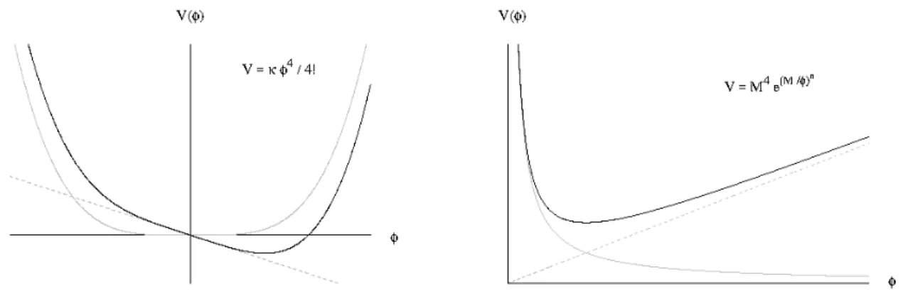
Figure 1.1: Depiction of how the chameleon potential (grey, solid) and its coupling to matter (grey, dotted)

combine into an effective potential (black) in two models: the exponential (right) and quartic (left) potentials.

The slope of the matter contribution becomes steeper in areas of higher density. In both potentials the

minimum is pushed toward lower values of

φ

and the curvature around the minimum increases as density

increases.

potential around its minimum,

m

=

d

_V

dφ

φ=φmin

,

(1.7)

is also dependent on the environment, increasing enough in regions of high density to suppress the field’s

ability to mediate a long-range force. Because of this ability to hide within its environment, the chameleon

can couple to matter with gravitational strength and still evade experimental detection in laboratory and Solar

System tests of gravity.

The vast majority of cosmological investigations of chameleon gravity have considered potentials of

the runaway form, such as the exponential

V

(φ) =

M

exp[(M/φ)

]

and power-law

V

(φ) =

M

φ

potentials. In order to evade Solar System tests of gravity,

M

has to be set to a value of

∼

10

eV, which is

the energy scale of dark energy [24]. This coincident energy scale gave the chameleon a lot of attention early

on as a possible explanation for cosmic acceleration. However, it was shown in Ref. [25] that the chameleon

field cannot account for the accelerated expansion of the Universe without including a constant term in its

potential. Nevertheless, light scalar fields arise in many theories that consider physics beyond the Standard

Model (SM), and the chameleon mechanism remains one of the most-studied approaches to screening the

unwanted forces mediated by these fields.

[29] have already placed constraints on chameleon theories. Additional experiments have been proposed:

one aims to measure the interactions between parallel plates to search for new forces [30] and another

suggests using atom interferometry between parallel plates of different densities to detect density-dependent

chameleon forces [31]. Laboratory searches for chameleon particles converted from photons in the presence

of a magnetic field via the Primakov effect have placed constraints on the chameleon-photon coupling [32, 33].

The CERN Axion Solar Telescope searched for chameleons created in the Sun by this effect [34] and is

currently conducting more sensitive searches [35] to detect solar chameleons via their radiation pressure [36].

Chameleon theories have also been constrained by their effects on the pulsation rate of Cepheids [37] and

comparisons of x-ray and weak-lensing profiles of galaxy clusters [38, 39]. There have also been efforts

to constrain the parameters of chameleon models by their effects on the cosmic microwave background

[40, 41], though these analyses focus specifically on potentials of the power-law form. Given the tremendous

experimental effort under way to detect or constrain chameleons, it is troubling that the most widely studied

chameleon models have been shown to suffer a breakdown in calculability in the early Universe due to the

discrepancy between the chameleon mass scale and that of the SM particles [42, 43].

In Chapter 2, we aim to identify a chameleon potential that can avoid the computational breakdown

suffered by runaway models. We analyze a class of potential not often considered in chameleon theories:

the quartic potential,

V

(φ) =

κφ

/4!

. Prevalent in high-energy theories, the quartic potential is also viable

as a chameleon model because the self-interaction of this potential is sufficient to ensure that the field will

be adequately screened in high-density environments [44]. The scale-free property of the quartic model is

potentially beneficial as it can avoid the hierarchy of energy scales that arises due to the low-energy scale of

the runaway potentials, and we investigate whether it is able to remain well-behaved in the early Universe.

Following our investigations in Chapter 2 into chameleon gravity, in Chapter 3 we turn our attention to

dark matter. While we do not yet know the nature or composition of dark matter, our wealth of cosmological

investigations allows us to put constraints on its origins. One of the most common origin stories for dark

matter is to assume that it was once in thermal equilibrium with SM particles in the early Universe. As the

SM plasma cooled, thermal production of dark matter ceased while annihilations continued. The dark matter

abundance thus began decreasing with the expansion until its annihilation rate equaled the Hubble rate, at

2_{Another proposed way to avoid the detrimental effect of the kicks is to include DBI-inspired corrections to the chameleon’s}

which point annihilations also ceased, and the dark matter abundance became constant. A second common

assumption is that this process, what we call dark matter freeze-out, occurred during a period in which the

energy density of the Universe was dominated by radiation. These assumptions allow one to calculate the

annihilation rate that generates the currently observed dark matter abundance. The required annihilation cross

section is “miraculously” of the electroweak scale [46]. However, as we continually place more stringent

bounds on dark matter properties, while failing to receive signals from any direct [47, 48, 49] or indirect

[50, 51, 52, 53, 54, 55] searches, interest in alternatives to this commonly considered scenario grows.

Alternatives to the common scenario often challenge the assumptions that dark matter was in thermal

equilibrium with SM particles and that it froze out during an era of radiation domination, both of which,

while tenable, are not strictly necessary. A period of radiation domination is required at temperatures below

∼

3

MeV in order to be consistent with the successful predictions of light element abundances from BBN

[56, 57, 58]. Inflation, however, is believed to occur at energy scales that greatly exceed this temperature, and

the thermal history of the Universe between the two periods is entirely unconstrained. In the simplest scenario,

the inflaton decays into relativistic particles that come to dominate the energy density of the Universe, and an

era of radiation domination begins [59, 60]. The transition to a radiation-dominated era, known as reheating,

is usually assumed to occur at temperatures many orders of magnitude above

3

MeV. It is not necessary,

however, that this be the case - the reheating of the Universe can occur at any temperature between

3

MeV

and the energy scale of inflation, and it can be caused by a number of different mechanisms.

In many models, inflation ends when the scalar field that drives inflation begins oscillating in its potential

minimum before decaying. If these oscillations occur in a quadratic potential, the field behaves as pressureless

fluid, and the Universe is effectively matter dominated [61]. Similar scenarios occur when one considers the

scalar (moduli) fields that are a common component of string theories [62, 63, 64, 65, 66, 67, 68, 69]. These

oscillating fields naturally come to dominate the energy density of the Universe following the decay of the

inflaton, providing another viable mechanism to produce an effectively matter-dominated era. Hidden-sector

theories, in which the dark matter does not couple directly to the SM, can also alter the thermal history

[70, 71, 72, 73, 74, 75], providing yet another means to achieve a period of matter domination prior to BBN.

Thus, an early matter-dominated era (EMDE) arises in many theories of the early Universe.

if dark matter thermally decoupled during the EMDE, a smaller annihilation cross section

h

σ

v

i

is required

to compensate for this dilution and provide the observed dark matter abundance. Contrarily, if dark matter

is a decay product of the dominating component, its abundance can be significantly enhanced, requiring a

larger

h

σ

v

i

to compensate for the excess, a scenario already under pressure by

γ

-ray observations [93, 94].

The correct relic abundance can almost always be obtained with the appropriate combinations of

h

σ

v

i,

dark matter branching ratio, and temperature at reheating [80, 81, 85, 90]. In many scenarios, the dominant

production mechanism for dark matter is by decay, rather than thermal production.

Another interesting consequence of an EMDE is the growth of small-scale structure. Subhorizon density

perturbations in dark matter grow linearly with the scale factor during an EMDE, as opposed to the much

slower logarithmic growth experienced during a radiation-dominated era [95, 96, 97]. This linear growth can

provide an enhancement to dark matter structure on extremely small scales (

λ

.

30

pc for temperature at

reheating

>

3

MeV), providing observable consequences to this scenario if dark matter is a cold thermal relic

[97, 98, 99].

However, if the dark matter is relativistic at reheating, the perturbation modes that enter the horizon

during the EMDE will be wiped out by the free streaming of dark matter particles [95, 96]. For this reason,

Ref. [95] assumed that the dark matter particles were born from the decay process with nonrelativistic

velocities or had a way of rapidly cooling in order for the enhancement to substructure to be preserved.

Assuming a nonrelativistic initial velocity for the dark matter requires a small, finely tuned mass splitting

between the parent and daughter particles, and it is more natural to assume any daughter particles are produced

relativistically.

Reference [96] claimed that the large free-streaming length of dark matter produced relativistically

from scalar decay would washout any enhancement to structure growth. However, Ref. [96] reached this

conclusion by assuming that all dark matter particles were created at reheating, neglecting those particles

created during the EMDE. The momenta of particles born prior to reheating decreased throughout the EMDE.

Consequently, particles born earlier will be slower at reheating. In Chapter 3, we investigate the extent to

which the redshifting of the particles’ momenta affects their velocity distribution at reheating, focusing on

the average particle velocity and the fraction of particles below a given velocity, to determine under what

conditions the EMDE enhancement to structure growth can be preserved.

power spectrum at the smallest observable scales,

0.5Mpc/h < λ <

20Mpc/h

[100, 101, 102] by measuring

the line-of-sight distribution of hydrogen gas clouds through their absorption of

Lyman

−

α

photons from

distant quasars. The Milky Way’s (MW) satellite galaxies also constrain the small-scale power spectrum

[103]. Preventing the suppression of power at these scales provides us with constraints on the allowed dark

matter velocity at its production for a given reheat temperature.

In Chapter 4 we consider how including scattering interactions between the dark matter and SM particles

could effect our constraints. If dark matter can efficiently transfer momentum to SM particles it has a way to

rapidly cool after its production. In Chapter 3, however, we show the vast majority of particles are produced

near reheating. Thus if the dark matter decouples from the SM early in the EMDE, very few dark matter

particles are ever able to interact with the SM and results from the noninteracting case are still largely

applicable. If dark matter remains coupled to the SM well after reheating, then the dark matter acquires the

standard thermal velocity distribution and all record of its nonthermal history is lost. Interactions between

dark matter and the SM only leave a distinctive impact on the dark matter velocity distribution function when

the decoupling occurs at or near reheating. In Chapter 4, we explore to what extent our constraints can be

relaxed if these interaction are included.

CHAPTER 2

Dark Energy:

Quartic Chameleons

1

_{In the commonly-considered runaway chameleon models, the field rolls to some value far from the}

minimum of its effective potential after inflation and remains stuck there during the radiation-dominated era

due to Hubble friction. The chameleon’s coupling to the trace of the stress-energy tensor makes it sensitive to

the energy density,

ρ

, and pressure,

P

, of the radiation bath through the quantity

Σ

≡

(ρ

−

3P

)/ρ

. While the

Universe is radiation dominated,

Σ

is nearly zero and the chameleon is light enough that Hubble friction is

able to prevent it from rolling toward its potential minimum. However, as the temperature of the radiation bath

cools, particle species in thermal equilibrium become nonrelativistic and

Σ

momentarily becomes nonzero.

The chameleon then gains mass, is able the overcome Hubble friction, and is seemingly “kicked” toward the

minimum of its effective potential [104].

Originally, the kicks were seen as an auspicious way to bring runaway chameleons to their potential

minimum prior to Big Bang Nucleosynthesis (BBN).

_{However, they impart such a high velocity to the field}

that the chameleon rebounds off the other side of its effective potential back to field values further from the

potential minimum than where it was stuck when the kick began [105]. However, Ref. [105] also showed

that the inclusion of a coupling between the chameleon and the electromagnetic field offers a solution. The

chameleon’s coupling to a primordial magnetic field allows the chameleon to overcome Hubble friction and

begin oscillating about its potential minimum prior to the kicks. For a sufficiently rapidly oscillating field, the

kicks then have little effect on the chameleon’s evolution.

These kicks further jeopardized chameleon theories by throwing into question their validity as a classical

field theory [42, 43]. The effective potential in runaway models is minimized when

φ

∼

M

, and at field values

φ

.

M

, the extremely steep slope of the bare potential leads to rapid changes in the chameleon’s effective

The contents of this chapter have been published as an article in Physical Review D. The original citation is as follows: Carisa

Miller and Adrienne Erickcek. Quartic Chameleons: Safely Scale-Free in the Early Universe.Phys. Rev.D94:104049, 2016.

2_{A consequence of the chameleon’s coupling to matter is that any variation in the chameleon field can be recast as a variation}

mass for small field displacements. Thus, the GeV-scale velocity with which the chameleon approaches its

meV-scale minimum after the kicks causes nonadiabatic changes in the mass that excite extremely energetic

fluctuations and lead to the quantum production of particles [42, 43]. Quantum corrections due to particle

production then invalidate the classical treatment of the chameleon field and the particles’ trans-Planckian

energies cast doubt on the chameleon’s viability as an Effective Field Theory (EFT) at the energy scale of

BBN.

We will show that the quartic potential is able to avoid these problems due to its scale-free nature. In the

early Universe, a chameleon field in a quartic potential oscillates rapidly with a large amplitude far beyond

the minimum of its effective potential. In the classical treatment, the chameleon would continue this behavior

until the end of radiation domination and still be oscillating far outside its minimum at the onset of BBN.

A quantum treatment of the chameleon’s motion shows that these oscillations will create particles, albeit

with much less energy than those created during the rebounds off runaway potentials. The same quantum

effects that were catastrophic to previous chameleon models will cause the field to lose energy and bring

the quartic chameleon to its potential minimum prior to the onset of the kicks. Consequently, for the quartic

chameleon, these kicks do not have as significant an influence on the field’s evolution as in models with

runaway potentials. Depending on the value of

κ

, the rate at which the field loses energy can vary significantly.

For large values of

κ

, the field can lose all of its initial energy to particle production within the first oscillation

and fall to its minimum. However when

κ

is closer to unity only a small percentage of the energy is lost

during each oscillation, but the total effect accumulates over many oscillations to introduce a decay factor to

the amplitude that still allows the field to reach its potential minimum before the kicks.

2.1

Classical Chameleons

In theories of chameleon gravity, the action can be written as

S

=

Z

d

x

√

−

g∗

M

2

R∗

−

1

2

(

∇

2

₋

_V

_(φ)

+

S

[˜

g

, ψ

]

,

(2.1)

where

g∗

is the determinant of the metric

g

that solves the Einstein equations,

R∗

is its Ricci scalar, and

V

(φ)

is the potential of the chameleon field,

φ

. The spacetime metric

˜

g

that appears in the action for the

matter fields,

S

, governs geodesic motion and is conformally coupled to the Einstein metric by

˜

g

=

e

g

,

(2.2)

where

β

is a positive, dimensionless coupling constant assumed to be of order unity.

This coupling

implies that the Einstein-frame stress-energy tensor of the matter fields is

T

=

e

T

˜

. With this

relationship between

T

and

T

˜

, the Einstein and Jordan frame energy density and pressure can be related

by

ρ∗

/˜

ρ

=

P∗/

P

˜

=

e

_{. It follows that any quantity that is a ratio of elements of the stress energy}

tensor, such as

Σ

or

w

≡

P/ρ

, is the same in both frames and can be evaluated using either Einstein- or

Jordan- frame quantities.

Varying the action with respect to

g

implies that

T

is not conserved in the Einstein frame, as

energy is exchanged between matter and the chameleon field. However, as the scalar and matter fields do

not interact in the Jordan frame, the Jordan-frame stress-energy tensor is conserved:

∇

˜

T

˜

= 0

. In a

Friedmann-Robertson-Walker spacetime, the scale factors in the Jordan and Einstein frames are related by

˜

a

=

e

_a∗

_{and the proper times are related by}

_d

˜

_t

₌

_e

_dt∗

_{. Since the Einstein-frame matter}

density is not conserved, it does not follow the usual

a

∗

scaling. Radiation, however, still follows the

expected

a

behavior. To show this, we begin by writing the conservation equation in the Jordan frame,

˜

ρ

∝

a

˜

.

(2.3)

3_{In most other chameleon theories, the bare potential and the matter coupling term must slope in opposite directions in order to}

produce the required minimum in the effective potential, and the coupling is generally given with a positive exponential. However, for the quartic potential, the coupling may slope in either direction and still produce a minimum, so in following with Ref. [44] we

Exchanging the Jordan frame quantities for those of the Einstein frame, we have

ρ∗e

_∝

a∗e

,

ρ∗e

_∝

_a

∗

e

,

ρ∗e

_∝

_a

∗

.

(2.4)

For matter we have

w

= 0

and Eq. (2.4) becomes

ρ∗

e

∝

a

.

(2.5)

Clearly, the Einstein-frame energy density in matter,

ρ∗

, does not scale as

a

. This follows from our earlier

statement that the stress-energy tensor that is conserved in the Einstein frame is not

T

, but the sum of

T

and the stress-energy tensor of the chameleon field. Often it has been the practice to define the left-hand side

Eq. (2.5) as the matter density as it is the quantity that follows the conservation equation in the Einstein frame

[24, 104].

For radiation, however,

w

= 1/3

and we find from Eq. (2.4) that

ρ∗

∝

a

.

(2.6)

In both frames the energy density in radiation is proportional to

a

∗

, and it follows that

H∗

∝

a

.

Throughout the remainder of the work we will drop the

∗

subscript on the scale factor when discussing how

quantities scale in the Einstein frame.

The relationship between

T

and

T

˜

also implies that the Jordan-frame temperature,

T

, depends on

φ

. As entropy is conserved in the Jordan frame,

g∗

(T

) ˜

a

T

is constant, and the expression for

T

in terms

of

φ

and

a∗

is

T

[g∗

(T

)]

= [g∗

(T

)]

T

e

a∗

a∗

.

(2.7)

2.1.1

Chameleon Cosmology

Varying the action with respect to the field

φ

gives the equation of motion for the chameleon:

¨

φ

+ 3H∗

φ

˙

=

−

dV

dφ

−

β

M

T

;

(2.8)

=

−

dV

dφ

+

β

M

(ρ∗

−

3P∗),

(2.9)

where the dot denotes a derivative with respect to proper time

t∗

in the Einstein frame and

H∗

≡

a∗/a∗

˙

.

The effective potential that controls the evolution of the chameleon field is

V

(φ) =

V

(φ)

−

βφ

M

(ρ∗

−

3P∗);

(2.10)

=

κ

4!

φ

4

₋

βφ

M

Σρ∗,

(2.11)

where

κ

is a dimensionless constant, and we have used the definition

Σ

≡

(ρ∗

−

3P∗)/ρ∗

. Quantum loop

corrections to the classical potential and limits on fifth forces constrain

β

and

κ

. The chameleon mechanism

depends on an increase in the chameleon’s effective mass in order to hide its effects, however quantum

corrections to its potential also increase with its mass. Maintaining the reliability of fifth-force predictions

requires that these corrections remain small compared to the classical potential and places an upper limit on

the chameleon mass that implies

κ

.

100

[106]. Laboratory searches for fifth forces, in turn, have already

placed lower bounds on the chameleon mass, which can to used to constrain

κ

from below for given

β

[107].

In order for

κ

to be of order unity, the chameleon coupling must be

β

.

10

. Conversely, in order for

β

to

be of order unity,

κ

must be

&

50

.

The minimum of this effective potential,

φ

=

6βΣρ∗

κM

,

(2.12)

is dependent on

ρ∗

and on

P∗

through the definition of

Σ

, and so, too, is the chameleon’s effective mass

m

=

d

V /dφ

φ=φmin

. The mass increases with

ρ∗

, making the chameleon heavier in regions of high

density and unable to mediate a long-range force.

When evaluating the chameleon equation of motion, we work with a dimensionless scalar field

ϕ

≡

variable

p

and the first Friedmann equation is

H

=

ρ∗

+

V

3M

Pl

[1

−

(ϕ

)

/6]

.

(2.13)

Using the above equation and the fact that

Σ

1

during radiation domination and

V

(φ)

ρ∗

, the chameleon

equation of motion, Eq. (2.9), can be written as

ρ∗

+

V

[1

−

(ϕ

)

_/6]

ϕ

00

₌

₋

_ϕ

_(ρ∗

_{+ 3V}

₎

₋

₃

dV

dϕ

−

βΣρ∗

.

(2.14)

We will use this equation in order to explore the evolution of a chameleon field in a quartic potential

throughout the radiation-dominated era.

The initial conditions for Eq. (2.14) follow from the field’s dynamics prior to reheating. During inflation,

the equation of state parameter

w

is approximately

−

1

, and the comparatively large value of the kick function,

Σ = (1

−

3w)

'

4

, sets the value of

φ

drastically greater than it is during radiation domination. The mass

of the field at its minimum is

m

=

κ

2

φ

=

9

2

κβ

Σρ∗

M

.

(2.15)

When

Σ

&

1

, the response time of the field

m

is much shorter than the Hubble time

H

as long as

ρ∗

M

,

m

H

'

3

9

2

κβ

Σ

M

ρ∗

.

(2.16)

Therefore, the field is massive enough to roll to its minimum prior to the onset of radiation domination. The

fact that

m

H

also implies that the chameleon field is massive enough during inflation that quantum

effects do not generate superhorizon perturbations in its value.

During reheating, the energy density

ρ∗

(be it of the inflaton or another oscillating scalar field) is converted

into radiation. The value of the kick function then drops to

Σ

1

, and

φ

is pushed to significantly

smaller field values; see Eq. (2.12). For all reheat temperatures much less than

M

we can assume that the

chameleon begins at rest with

φ

equal to the value of

φ

just prior to the drop in

Σ

, because

m

H

, as

is 0.001 [108].

Σ

then maintains this value until

T

'

600

GeV when contributions from massive particles

become comparable. As the temperature decreases,

Σ

begins to increase as

Σ

∝

m

/T

, where

m

is the

mass of the most massive SM particle species: the top quark [108].

At

T

'

200

GeV the process that gives the kick function its name begins. As the temperature of the

radiation bath decreases, the energy density and pressure of massive particles decay at slightly different rates,

allowing

Σ

to reach non-negligible values. This happens as each SM particle becomes nonrelativistic, but

contributions from some species merge together, and the entire process results in four distinct kicks. The

contributions from each particle are suppressed by a factor of

g∗(T

)

, where

g∗(T

)

is the effective degrees

of freedom. As the temperature cools,

g∗

(T

)

decreases, and each kick becomes larger than the last with the

final kick due to the electrons reaching a value of

Σ

'

0.1

. For a detailed calculation of the kick function

Σ

,

see Appendix A of Ref. [43].

2.1.2

Quartic Chameleons

For the runaway potentials usually considered in chameleon gravity, the value of

V

(φ)

approaches

infinity as

φ

→

0

and drops off rapidly as

φ

increases. The effective potential is then dominated by

V

(φ)

near

φ

= 0

and by the linear matter-coupling term at field values greater than

φ

. During inflation, the

large value of

Σ

makes the slope of the matter-coupling term in Eq. (2.10) steeper, and the chameleon sits

in a potential minimum at a small

φ

value. When inflation ends and

Σ

decreases, the slope of the matter

contribution to

V

becomes shallow and the minimum of the effective potential moves to larger values of

φ

.

The chameleon then rolls down its bare potential, past the minimum, and out to where the effective potential

is dominated by the matter-coupling term. The field then becomes stuck due to Hubble friction until it is

kicked back toward the minimum of its effective potential.

The quartic chameleon, however, feels the effects of its bare potential on both sides of the minimum of

its effective potential. As previously discussed, the comparatively large value of

Σ

prior to reheating fixes

φ

at a large value far from zero. Throughout this analysis, we use the subscript

i

to indicate the value of a

quantity just prior to the onset of radiation domination, which we take to occur at a Jordan-frame temperature

T

= 10

GeV. The value of

φ

is then

φ

'

0.0062M

β

κ

We have also assumed an era of inflation prior to radiation domination and have therefore used

Σ

= 4

.

However, nonstandard histories can easily be accounted for by changing this value in Eq. (2.12). We will show

that the values of

Σ

and

T

, only set the initial oscillation amplitude of the field, to which the subsequent

evolution is largely insensitive.

When the value of

Σ

drops from

4

to

0.001

at the end of inflation, the value of

φ

decreases by a

factor of

(0.001/4)

'

0.06

. The chameleon then rolls rapidly down its bare potential toward this new

minimum. In its decent to its potential minimum, the chameleon gains sufficient energy that the slight tilt at

the bottom of the quartic well due to the now small matter coupling does very little to affect its motion as it

passes through

φ

and climbs up the other side of its bare potential. It climbs to almost the same potential

value as it started before turning around and falling again with nearly the same energy. It continues in this

fashion, oscillating back and forth, all but oblivious to the matter coupling.

The oscillation amplitude decreases as Hubble friction causes the energy in the chameleon field to

redshift away as

a

. This behavior can be understood easily by the virial theorem. For a general power-law

potential of the form

V

(φ) =

Cφ

, the virial theorem relates the rapidly oscillating field’s average kinetic

and potential energies,

K

and

V

, by

2 ¯

K

=

n

V .

¯

(2.18)

The equation-of-state parameter

w

is then

w

=

P

¯

¯

ρ

=

1 2

φ

˙

−

V

φ

˙

+

V

=

n

−

2

n

+ 2

.

(2.19)

Using this value of

w

, we can determine how the chameleon energy will scale with expansion by using the

conservation equation:

ρ

=

ρ

a

;

=

ρ

a

2n

n+2)

_.

_(2.20)

-0.002 -0.001 0 0.001 0.002

φ

/ M

pl

0

1x1061

2x1061

3x1061

4x1061

5x1061

6x1061

7x1061

8x1061

0 0.1 0.2 0.3 0.4 0.5 0.6 0.7 0.8

Energy Density [GeV

4 ]

p = ln(a/a_i)

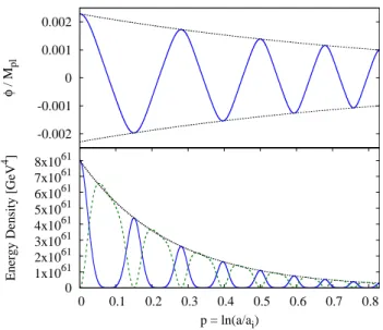
Figure 2.1: Top: The value of

ϕ

(blue, solid) and the values of its minima and maxima,

−

ϕ

a

and

ϕ

a

,

respectively (black, dotted) over the course of four oscillations. Bottom: The kinetic (green, dashed) and

potential (blue, solid) energies of the chameleon and their amplitude,

V

a

(black, dotted). The potential

energy reaches a maximum twice during each complete oscillation when

|

ϕ

|

is at a maximum. The kinetic

energy reaches its maxima both times

ϕ

passes through

ϕ

. At all times the chameleon energy density is

much less than that of the radiation

ρ∗

∼

(T

a

)

= 10

a

GeV (In this and all figures

β

= 0.1

and

κ

= 2

.)

matter. However, we will show later in Section 2.2.2 that the corrections to the evolution of the chameleon’s

energy density are negligible.

As the energy in the chameleon field is the sum of its kinetic and potential energies, the maximum

values of both of these quantities during each oscillation will scale as

a

. The potential energy of the

field when it reaches the peak of each oscillation,

V

, and its kinetic energy each time the field passes

through the minimum of its potential,

K

= ˙

φ

/2

, are both related to the field’s initial potential energy

by

V

=

K

=

V

a

. The quartic relation between

φ

and

V

implies that the amplitude of the

φ

oscillations decays as

a

, so the value of

φ

at the peak of each oscillation is

φ

=

φ

a

. Both of

these behaviors can be seen in Figure 1, which shows the value of

ϕ

in the top panel and the kinetic and

potential energy of the field in the bottom panel plotted over the course of several oscillations. These plots

are generated from the numerical solution to Eq. (2.14) assuming

ϕ

= 0

and

ϕ

=

φ

/M

with

β

= 0.1

and

κ

= 2

.

The fact that the quartic chameleon begins at

φ

M

and does not exceed this value is an interesting

friction can be nearly equal to

M

[104]. If the field remains stuck at such values until BBN, the large

variation of

φ

from its potential minimum can be interpreted as a larger variation in particle masses than we

know to be allowed. Quartic chameleons, however, are already at field values much less than

M

before the

end of inflation and oscillate with a decreasing amplitude. While we will show that the field still finds its

minimum prior to the kicks, it is not strictly necessary to avoid endangering the success of BBN.

Equation (2.12) implies that

φ

is proportional to the cube root of the energy density in radiation

and so will decay as

a

_{. Thus,}

_φ

min

will decrease faster than the oscillation amplitude by a factor of

a

, implying that the value of

φ

at the maximum of its oscillations will always exceed the minimum

of its effective potential. Therefore, our classical treatment of the chameleon’s behavior suggests that it

would spend most of its time in regions dominated by its bare potential far from the minimum of its effective

potential (though not far enough to significantly effect particle masses), allowing the oscillations to continue

indefinitely while the Universe is radiation dominated. The high-energy oscillations of the field prevent

it from becoming stuck due to Hubble friction or falling into and tracking its minimum. However, as the

problems with other chameleon models demonstrate, the quantum effects associated with rapid changes in

the chameleon field can significantly alter this classical behavior.

2.2

Quantum Chameleons

In chameleon models with runaway potentials, the only instances of rapid changes of the chameleon field

after inflation occur when the chameleon is kicked toward its potential minimum with a very high velocity

and rebounds off its steep bare potential. The rapid changes in the mass of the chameleon during this rebound

excite high-energy perturbations that, in a naive, classical evaluation, exceed the energy initially available

to the chameleon field. Considerations of the backreaction of particle production on the field showed that

quantum corrections significantly alter the form of the potential experienced by the chameleon field. These

corrections radically change the chameleon’s evolution throughout the rebound, causing it to turn around

long before it would have exhausted the kinetic energy it possessed going into the rebound, which keeps the

occupation numbers of the excited modes extremely small [43].

results Ref. [106], which also used quantum corrections to place an upper bound on

κ

. For the relatively

large values of

κ

near this limit, the field can lose all of its initial energy to particles before it completes an

oscillation, and it simply falls to its potential minimum. For smaller values (

κ

.

O

(1)

), the energy lost is

only a small fraction of the field’s energy at the start of an oscillation, and the evolution of the field over a

single oscillation is not significantly altered. Instead, this energy loss accumulates over many oscillations

and introduces an additional decay factor to the oscillation amplitude causing it to decay faster and reach its

potential minimum.

2.2.1

Particle Production

We first summarize how rapid changes in the chameleon’s effective mass excite perturbations [109]; for

a more detailed review of this process, see Appendix C of Ref. [43]. We begin by decomposing the field into

its spatial average

φ(t)

¯

and the perturbation

δφ

:

φ(t,

x) = ¯

φ(t) +

δφ(t,

x).

(2.21)

The linearized perturbation equation that governs the evolution of

δφ

is

∂

+ 3H∂

−

∇

a

+

V

( ¯

φ)

δφ

= 0.

(2.22)

Throughout this section we will not be using the variable

p

, and primes will denote differentiation with

respect to the argument of the function.

To quantize the perturbations, we introduce the creation and annihilation operators

ˆ

a

and

ˆ

a

, respectively,

which obey the standard commutation relations,

h

ˆ

a

,

ˆ

a

i

= (2π)

δ

k

−

k

.

(2.23)

The annihilation operator annihilates the vacuum state:

ˆ

a

|

0

i

= 0

. Using

ˆ

a

†

k

and

ˆ

a

we can then express

δφ(τ

)

as

ˆ

δφ(τ,

x) =

Z

d

k

(2π)

ˆ

a

φ

(τ

)

a(τ

)

e

ik·x

_{+ ˆ}

_a

k

φ

(τ

)

a(τ

)

e

−ik·x

where

τ

is conformal time. Inserting this decomposition of

δφ

into Eq. (2.22), we find

φ

(τ

) +

ω

(τ

)φ

= 0;

(2.25)

ω

(τ

) =

k

+

a

V

( ¯

φ)

−

a

00

_(τ

₎

a

,

(2.26)

where

ω

(τ

)

is the effective mass of a plane-wave perturbation in the chameleon field with a comoving

wavenumber

k

.

During radiation domination

a

(τ

) = 0

, and

ω

=

k

+

a

V

φ

¯

'

k

+

κ

2

(a∗φ)

2

_,

_(2.27)

where in the last equality we have dropped the bar over

φ

as we will be working exclusively with the spatially

averaged field. We also neglect the matter coupling because it is subdominant to the bare potential throughout

most of the oscillation. When

ω

(τ

)/ω

&

1

, perturbations in the field are excited. Taking the derivative of

this effective mass with respect to

τ

, we find

ω

(τ

) =

a

2ω

h

2H∗V

(φ) +

V

(φ) ˙

φ

i

;

=

a

2ω

h

κH∗φ

+

κφ

φ

˙

i

.

(2.28)

We can simplify the last line of the equation by noting that not only is

H∗φ

_{initially smaller than}

_φ

_φ

˙

_{, it}

also redshifts away faster. This can be seen by recalling the relations

φ

=

φ

a

,

φ

˙

=

√

2K

=

√

2V

a

, and using the fact that, during radiation domination,

H∗

decreases as

a

. With these results, the

maximum value of the first term during each oscillation is

H∗φ

'

H∗

φ

a

. The second term, however,

is a product of two oscillating functions that reach their maxima at different times. From the approximately

sinusoidal nature of

φ

, we can determine that the product of

φ

and its derivative

φ

˙

will behave as the product

of their amplitudes and another sinusoidal function, thus,

(φ

φ)

˙

is proportional to

φ

φ

˙

. The constant

of proportionality can be numerically determined and is

≈

0.6

for all

β

and

κ

. The amplitude of the second

term is then

(φ

φ)

˙

∼

φ

φ

˙

'

φ

a

√

2K

'

p