honors-thesis04052017-final.pdf

EXTENDING

DYNAMIC

TREATMENT

REGIMES TO

INCORPORATE

L

D

O

B

D

T

Mengbing Li

Senior Honors Thesis Department of Biostatistics

University of North Carolina at Chapel Hill 2017

Approved by:

Dr. Michael Kosorok, Thesis Advisor,

Dr. Jane Monaco, Reader,

ABSTRACT

MENGBING LI: Extending Dynamic Treatment Regimes to Incorporate Longitudinal Data Observed Between Decision Times.

(Under the direction of Dr. Michael Kosorok, Thesis Advisor)

ACKNOWLEDGMENTS

I would first like to thank my parents who have offered me emotional and financial support throughout college. Without them I may not have found myself at UNC, nor had the courage to pursue whatever subjects I enjoy or to engage in this task.

Importantly, I would like to thank my thesis advisor Professor Michael Kosorok, for the guidance and advice throughout the process of writing the thesis. I am very grateful for the precious time and extraordinary patience he offered me when helping me learn the very basics of machine learning and its applications in clinical trials, guiding me to read and understand research papers, helping me narrow down my thesis topic, and providing insights and editorial support for my writing. Thank you Dr. Kosorok, for showing an interesting brand new research area to me and giving me a good taste of research.

Next, I would like to thank both Professor Gary Koch and Professor Jane Monaco. Since my junior year, Dr. Koch has been providing me a position at the Biometrics Con-sulting Lab, where I had the opportunity to get involved in statistical projects that allowed me to practice the knowledge I learned from classes in real world settings. He has also of-fered me numerous useful and insightful suggestions on course selection, career planning, and graduate school applications. I have known Dr. Monaco since my sophomore year, and it was she and her passion that initially inspired me to pursue biostatistics. Without her generous help and invaluable advice throughout the past three years, my study at UNC would not have been so smooth and enjoyable.

Lastly, thank you to my friends and roommates for bringing me wonderful life expe-riences. Thank you to my professors in the STOR department who I have taken classes with and who attract me to the wonderful world of statistics. Finally, a big thank you to UNC-Chapel Hill, of which I am always proud being a Tar Heel.

TABLE OF CONTENTS

LIST OF FIGURES . . . vi

1 INTRODUCTION . . . 1

2 DATA SETTINGS AND NOTATIONS . . . 5

2.1 Standard Settings . . . 5

2.1.1 Individualized Treatment Rule in Standard Single-Stage Settings . . . 5

2.1.2 Dynamic Treatment Regimes in Standard Multi-Stage Settings. . . 5

2.1.3 Observational Setting . . . 8

2.2 Dynamic Treatment Regimes (DTRs) with Additional Longitudinal Data . . . 9

2.2.1 Regularly Spaced Data . . . 9

2.2.2 Irregularly Spaced Data. . . 11

3 REINFORCEMENT LEARNING . . . 13

3.1 Reinforcement Learning and Q-Learning Backgrounds . . . 13

3.2 Estimating the Q-Function . . . 16

3.2.1 Support Vector Regression . . . 16

3.2.2 Extremely Randomized Trees . . . 18

3.3 Discussion . . . 18

4 OUTCOME WEIGHTED LEARNING . . . 19

5 BACKWARD AND SIMULTANEOUS OUTCOME WEIGHTED LEARNING . . . 23

5.1 Backward Outcome Weighted Learning (BOWL) . . . 23

5.2 Simultaneous Outcome Weighted Learning . . . 25

6 PROPOSED METHODOLOGY FOR ADDITIONAL LONGITUDINAL DATA . . 27 7 DISCUSSION . . . 31 8 REFERENCES . . . 33

LIST OF FIGURES

1 INTRODUCTION

Many clinical trials are designed to examine drug effects on the patient population as a whole in a single stage. However, this unchanged ”one-size-fits-all” scheme can be problematic in clinical practice because of heterogeneity of patient characteristics and dif-ferences in patient treatment progression. An ideal optimal treatment regime is expected to overcome such problems and be individualized and adaptive over time. For example, in treating patients with psychiatric disorders, clinicians need to consider individual character-istics which may influence treatment response. Considering the delayed treatment effects and potential reoccurrence of symptoms, clinicians may also want to relieve the waxing and waining of patients following long-term treatments, which significantly increase the risks of severe side effects, psychological and physical stress, as well as economic burden of pa-tients (Murphyet al.2006). Therefore, a tailored adaptive treatment design will contribute to both optimizing treatment effects as well as reducing patient burden.

clinical practice.

However, although DTRs require patient data collected at each decision point, patient status and disease progress are not constantly monitored between stages. Additional data within each stage over time, whether regularly or irregularly collected or not, may aid in finding better treatment regimes for patients. In a recently conducted study, researchers appealed to adaptive mobile health (mHealth) to help smokers quit (McClureet al.2016). In the study, participants randomized to an adaptive interactive program which provided real-time, adaptively tailored advice on top of standard self-help content, showed a higher proportion (76%) of quitting than participants randomized to an non-adaptive program with standard self-help content (67%). Thus mHealth can serve as a promising intervention to provide additional data along with treatment in that smart phones are capable of offering prompt feedback to both smokers and clinicians to make better tailored treatment decisions. Another example that illustrates the usefulness of collecting additional patient data be-tween stages is treatment for Type I diabetes (T1D). Young adults with T1D often strug-gle with glycemic control and weight management (Liu et al. 2010). Compared to other adults with T1D, those young adults are more likely to experience extra energy loss result-ing from glucosuria (Anderbroet al.2010), increased resting energy expenditure (Schober

to optimizing glycemic control and weight management.

Although the scheme may seem promising, carrying out such a process requires many efforts. On one hand, even though rapidly developing technologies greatly facilitate the data collection processes through, for example, smart phones, electronic wristbands, and other portable devices, there is no existing protocol specifying rules and restrictions of the data collection process. On the other hand, challenges of analyzing the data are significant. First, finding the optimal DTR usually requires machine learning methods. In (Zhao

et al.2009), the authors applied reinforcement learning, specifically Q-learning, to discov-ering the optimal treatment regime in clinical trials for life-threatening diseases. Q-learning is a model-free temporal difference learning algorithm that deals with infinite-state Markov Decision Processes (MDP). Rather than learning the MDP, Q-learning instead learns the value of each state and the optimal policy directly by only using existing states and avail-able actions in each state. The goal of Q-learning is to optimize the Q-function, which is the expected discounted reward after executing an action at the current state and following the policy in all states afterwards. Support vector regression and extremely randomized trees were used to estimate the Q-function. The method did not rely on precise dynamic mathematical models, and successfully incorporated delayed effects of treatments, drug efficacy, and drug toxicity into improving long-term clinical outcomes.

(Zhao et al. 2012) was among the first to use machine learning techniques for clas-sification in estimating optimal treatment rules. The authors proposed outcome weighted learning (OWL) in estimating individualized treatment rules (ITR) with binary options. The method directly finds the optimal ITR that maximizes the clinical outcome using prognostic variables without modeling the conditional means. (Zhao et al. 2015) proposed two new nonparametric machine learning methods for estimating the optimal DTR. One is called backward outcome weighted learning (BOWL), which treats estimating the optimal DTR as a sequence of weighted classification problems. It starts from the last stage, estimating

the optimal decision rule in future stages first and then the optimal decision rule in the pre-ceding stages by restricting analysis to patients who followed exactly all future treatment rules. The other is called simultaneous outcome weighted learning (SOWL), which sees estimating the optimal DTR as a single classification problem. It finds the optimal DTR by directly maximizing the expected average reward. All the above methods are useful in a standard DTR design, but may not be directly applicable to the newly proposed scheme where additional longitudinal data are collected between stages.

Second, since we would like to monitor real-time changes in patient status, it is very likely that data are collected at irregularly spaced time points and are distributed sparsely (Caoet al.2015). Given a patient, the sparsity refers to the small number of covariates and response variables that are observed at the same time, leading to asynchronous data and violating assumptions for standard methods for analyzing longitudinal data. Thus special methods such as the one proposed by (Caoet al.2015) should be considered.

2 DATA SETTINGS AND NOTATIONS

2.1 Standard Settings

2.1.1 Individualized Treatment Rule in Standard Single-Stage Settings

In the usual standard setting, we only collect patient data at a single time point. We denote available information of each patient as a tuple(Xn, An, Yn), wheren= 1, . . . , N,

and each tuple is an independent and identically distributed trajectory of(X, A, Y). Here X is ap-dimensional random vector of covariates. We consider a setting where treatment assignments A ∈ A are independent of patient covariates X, where A is the collection of treatments received. A can be of any form including binary, discrete, and continuous. Y is the observed clinical outcome, which may also be called the reward depending on the context, and is coded so that larger values correspond to better outcomes. We assume Y is bounded. LetD be the collection of all possible treatment rules. An individualized treatment rule (ITR) is a mapd :X → A. An optimal ITR, denoted asdopt_{, is a rule that}

maximizes the expected outcome if implemented by the entire population. Thus our goal is to quantify the relationship between(X, A, Y)so that the maximumY can be achieved. Depending on the type of treatment assignments, we can apply regression methods, such as the generalized linear regression, to establish the desired relationship.

2.1.2 Dynamic Treatment Regimes in Standard Multi-Stage Settings

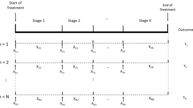
In a K-stage setting, we collect patient data atK decision time points. We can repre-sent each patient’s available information as(Xn1, An1, Xn2, An2, . . . , XnK, AnK, Yn)where

n = 1, . . . , N and each tuple is an independent and identically distributed trajectory of (X1, A1, X2, A2, . . . , XK, AK, Y)sampled at random from a distributionP. Here for each

collection of treatment assignments at stage k. Xk is the available patient information

after treatment assignment Ak−1 but prior to the kth stage. Y is the final outcome after all stages of treatments and is coded so that larger values correspond to better outcomes. Let Hk = (X1, A1, . . . , Ak−1, Xk) ∈ Hk be the history information up to stage k with

H1 =X1, andDkbe the collection of available treatments at stagek. A dynamic treatment

regime (DTR) is a sequence of decision rules d = (d1, . . . , dK) where each dk is a map

from Hk to Dk. Our goal is to find the optimal DTR dopt that maximizes the expected

average outcome if the rule is implemented by the entire population in the future (Zhao 2015).

We can formalize the process through potential outcomes. We will use lowercase let-tersakto denote the realized treatment at stagek. An overbar will be used to denote events

that happened in the past, and an underbar will be used to denote events that will happen in the future. Thus we haveak = (a1, a2, . . . , ak), andak = (ak, ak+1, . . . , aK). Note that

d =d. Let X∗(ak)be a patient’s potential covariate status at the start of stagek provided

the sequence of treatments(a1, a2, . . . , ak)was assigned. LetY∗(aK)be a patient’s

poten-tial outcome at the end of the study provided the sequence of treatments(a1, . . . , aK)was

followed. In the above framework, we can write h1 = x1, a1 = d1(x1), x2 = X∗(d1) = X∗(a1), h2 = (x1, a1, x2) = (x2, a1), a2 = d2(h2), x3 = X∗(d2) = X∗(a2), . . . , aK−1 =

dK−1(hK−1), xK =X∗(dK−1) = X∗(aK−1), hK = (xK, aK−1), aK =dK(hK)andY∗(aK) =

Y∗(d) = Y∗(d). Our optimal DTR will be a rule with the property_E{Y∗_{(d)} ≤}

E{Y∗(dopt)}

for anyd∈ {(d1, . . . , dK)|dk ∈ Dk}.

1. Causal consistency: we assume that the potential outcome under a sequence of ments is the same as the observed outcome under this sequence of assigned treat-ments. Mathematically we can express this assumption as for ∀k = 1, . . . , K, if Ak−1 =ak−1 thenXk=X∗(ak−1), and ifAK =aK thenY =Y∗(aK).

2. Sequential ignorability: we assume that given the history information of patient co-variates and treatment assignments up to stage k, the treatment assignment at the next stagek + 1 is independent of potential outcomes of the individual under any treatment options across all stages. Mathematically, we have ∀ak ∈ Ak, Ak ⊥⊥

{X1, X2∗(a1), . . . , XK∗(aK−1), Y∗(aK)} |HK.

3. Positivity: we assume that for any tuples of history information of patient covari-ates and treatment assignments up to stage k that have a positive probability to be observed, the corresponding treatment regime will have a positive probability to be observed. Mathematically, we have∀k ifP[Hk = (xk, ak−1)]>0, then with proba-bility 1P[Ak=ak |Hk]>0.

Figure 2.1: Standard data setting for dynamic treatment regimes

2.1.3 Observational Setting

Settings mentioned above are both experimental. However in many circumstances, observational data play a major role. For example, research on cancers and diabetes are not likely to involve human experimental data due to ethical issues, and thus studying on such diseases heavily rely on observational data. Electronic health record (EHR) provides insightful information for clinical diagnosis and clinical research but is also observational. There are multiple benefits of using observational data (Kidwell 2015). First, obtaining observational data is usually the first step to understand disease characteristics and treat-ment effects. Second, using observational data is less likely to be concerned with ethical problems, such as research on cancers. Moreover, observational data are generally cheaper to collect than experimental data. In addition, especially for rare disease, it is more feasible to use observational data considering the small number of patients.

in observational studies, we cannot guarantee that covariate history up to any stagekis fully available. Besides, statistical methods for adjusting for confounding may not be applicable to time-varying treatment. Furthermore, deriving unbiased estimates for observational data is subject to model specification, even though this assumption may be weakened if using doubly robust methods (Kidwell 2015).

Considering these issues with observational settings, in this thesis we only consider the simpler settings where the assumptions for standard statistical methods are nicely specified. 2.2 Dynamic Treatment Regimes (DTRs) with Additional Longitudinal Data

2.2.1 Regularly Spaced Data

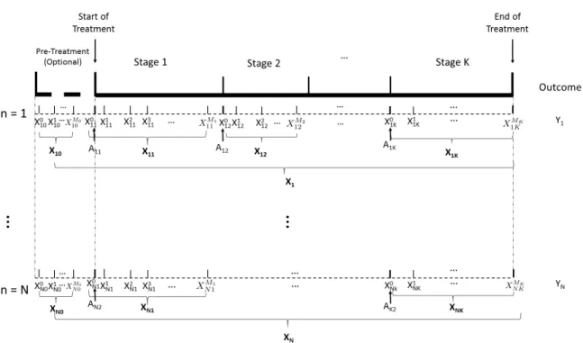
We consider a setting similar to DTRs with K stages except that additional data are collected across each stage. In addition to the treatment stages in a DTR, we allow an optional pre-treatment stage before stage one, which we will call stage 0. No treatment assignment is made in stage 0, but we may include preliminary patient data before the first treatment collected through electronic health record or mHealth etc. At each stage k = 0,1, . . . , K, patient data are collected atMkrandomly selected time points. Fork ≥1,

we usem = 0 to denote the time when covariates measured right after treatment Ank is

assigned to patientn. To simplify the notations, we also allowm= 0in the pre-treatment stage, even though no treatment assignments are made. We assume that covariates of all patients are measured at the same time, i.e. for eachk, we obtain information on covariates of each patientnatm = 0, . . . , Mk.

We use a p−dimensional vector Xm

nk to represent the available information of patient

n at time m in stage k. For patient n in stage k, the available covariate information is Xnk = (Xnk0 , . . . , X

Mk

nk )T. Data of all patients in stage k will be denoted as Xk =

(X1k,X2k, . . . ,XN k)T. LetYnbe the final clinical outcome which is coded so that larger

values correspond to better outcomes. Then similar to the standard DTRs, we can represent each patient’s information as(Xn0,Xn1, An1,Xn2, An2, . . . ,XnK, AnK, Yn)T where each

tuple is an independent and identically distributed trajectory of (X0, X1, A1, X2, A2, . . . , XK, AK, Y). Let Hk = (X0, X1, A1, . . . , Ak−1, Xk) ∈ Hk be the history information up

to stage k withH1 = (X0, X1), and Dk be the collection of available treatments at stage

k. A dynamic treatment regime (DTR) in this setting, similar to before, is a sequence of

decision rulesd= (d1, . . . , dK)where eachdkis a map fromHktoDk. Our goal is again

to find the optimal DTRdopt _{that maximizes the expected average outcome if the rule is}

implemented by the entire population in the future.

To formalize the process through potential outcomes, we can use the same notations as in standard DTRs, except thatx0 is added to all history variables. In addition, we make the same three assumptions for this modified setting, i.e. SUTVA, sequential ignorability, and positivity.

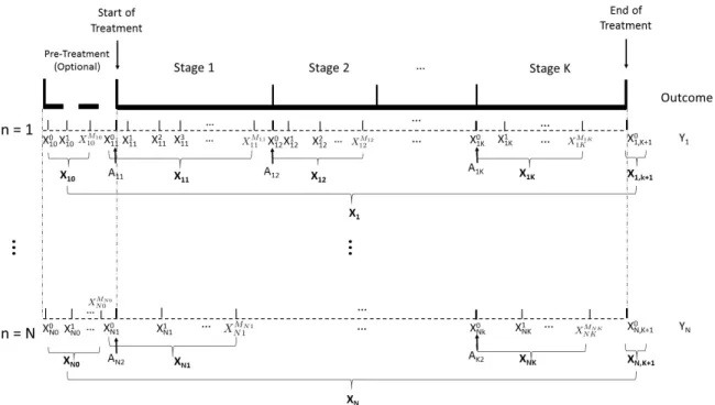
2.2.2 Irregularly Spaced Data

In real clinical practice, patients covariates are rarely measured at regular gaps. Instead, nearly all patients’ measuring time are different. Here we use irregularly spaced data to refer to the corresponding setting where at least one patient’s covariates are observed at a different time than other patients’ covariates, i.e. the data are asynchronous. In addition, given a stage, the number of observations for different patients may be different. Like the regularly spaced setting, we also allow stage 0, which is the optional pre-treatment stage before stage one. Suppose for patientn, we measure covariates at timemn= 0,1, . . . , Mnk

at stage k. For k ≥ 1, we use m = 0to denote the time when covariates measured right after treatmentAnkis assigned to patientn. To simplify the notations, we also allowm = 0

in the pre-treatment stage, even though no treatment assignments are made. As before, we use a p−dimensional vector Xmn

nk to represent the covariates of patient

n at time m in stage k. For patient n in stage k, the available covariate information is Xnk = (Xnk0 , . . . , X

Mnk

nk )T. Data of all patients in stage k will be denoted as Xk =

(X1k,X2k, . . . ,XN k)T. LetYnbe the final clinical outcome which is coded so that larger

values correspond to better outcomes. Then similar to the standard DTRs, we can represent each patient’s information as(Xn0,Xn1, An1,Xn2, An2, . . . ,XnK, AnK, Yn)where each

tu-ple is an independent and identically distributed trajectory of(X0, X1, A1, X2, A2, . . . , XK,

AK, Y). Although the proposed notations lead us to a similar situation to the previous one

where data are regularly spaced, it is dangerous to apply this simple data representation to our analysis because the data are too sparse for most existing methods to be valid.

Considering the small amount of literature dealing with this complicated situation, which is closest to the reality, most of our attention in this thesis will be paid to the pre-vious two multi-stage situations, where the data are not sparse or are regularly spaced for simplicity.

3 REINFORCEMENT LEARNING

We first review the statistical methods dealing with the standard DTRs. In treating life-threatening diseases such as breast cancer and lung cancer, many effective treatments involves multiple stages that are adaptive to patient performance. There are at least three challenges for statistical designs of adaptive treatment or trials. First, many existing designs are based on parametric models to account for efficacy, toxicity, and time to some events. For example, (Thallet al.2000) provided a statistical framework for multi-stage treatment or clinical trials with modifications of the play-the-winner-and-drop-the-loser strategy, in which a successful treatment is repeated while an unsuccessful one is replaced by another treatment. Second, as a result of the parametric models, the heterogeneity in treatment across individuals is ignored and the heterogeneity needed for optimizing individualized treatment rule is not incorporated. Third, long-term benefits of the treatment or trials are not successfully evaluated due to delayed effects. Considering these challenges, the authors of (Zhao et al. 2009) presented a general reinforcement learning framework and related statistical methods for discovering new treatment regimes.

3.1 Reinforcement Learning and Q-Learning Backgrounds

The basic idea of reinforcement learning is to maximize the outcomes, called the re-wards in this context, by telling the learning agent whether an action is “good” or “bad” when it tries among all available actions. In our DTR context, we useX andAto denote the space of patient covariates and the space of treatments respectively. In the reinforcement learning context, the random variablesXandAare called “state” and “action” respectively. Define the time-dependent random variables statesXk = {X0, X1, . . . , Xk}with realized

ak = {a0, a1, . . . , ak}. The state variables may or may not include past actions, i.e. Xk

may include Ak−1. The distribution P from which the finite longitudinal trajectories are randomly sampled consists of the unknown distribution of eachXkconditional on previous

(Xk−1, Ak−1)with conditional densities{f0, . . . , fK}. The expectations of the conditional

distributions with respect to the distribution P are denoted as E. For k = 0,1, . . . , K, we define the history information up to stagek for a patient asHk = (Xk, Ak−1). Define the outcome of a patient’s treatment after stage k asYk = R(Xk, Ak, Xk+1) = R(Hk+1) whereR is a (possibly random) map from the space of states and actions to the space of real numbers. The realized value of the reward after stagek isyk =R(xk, ak, xk+1). Our goal is to findakto maximize the expected discounted return:

˜

yk =yk+γyk+1+γ2yk+2+· · ·+γKyk+K = K−k

X

i=0

γiyk+i

whereγ ∈ [0,1]is the discount rate. Intuitively, ifγ is closer to 1, the future rewards are weighted more strongly.

A key element of the reinforcement learning framework is an exploration policy that maps past states and past actions to the probability that the next action a is taken given the past states and past actions, i.e. p : hk 7→ pt(a | hk). We can write dk(hk) = ak if

the policy is deterministic but not non-stationary wheredk is the decision rule in stagek.

Denote the distribution of training data asPdwhen the policydis used to generate actions,

and the corresponding expectations asEd. The optimal sequence of treatment, or optimal

policy here, maximizes the expectations with respect to the sum of the rewards over the time trajectories. We can represent our problem using a value function based on the state historyhk. The value function is the expected total future rewards of a patient conditional

onhk, i.e.

Vk(hk) = Ed

"_K−k X

i=0

γiYk+i |Hk=hk

#

Then the optimal value function is

V_k∗(hk) = max

d∈D Vk(hk) = maxd∈D Ed

"_K−k X

i=0

γiYk+i |Hk=hk

#

.

In reinforcement learning, value functions are supposed to satisfy some recursive relation-ships. Therefore we can write the optimal policydopt_as

dopt_k (hk)∈argmax ak

E

Yk+γVk∗+1(Hk+1)|Hk =hk, Ak =ak

.

In reality, it is common that the optimal policy is not directly computable, and there-fore the authors suggest using an alternative temporal-difference (TD) learning approach, specifically learning which estimates a function instead of the value function. Q-learning is an effective model-free algorithm that allows us to estimate the optimal strate-gies when we have insufficient knowledge about the distribution of the random variables. The optimal time-dependent Q-function is

Q∗_k(hk, ak) =E

Yk+γVk∗+1(Hk+1)|Hk=hk, Ak =ak

.

Since

V_k∗(hk) = max ak

Q∗_k(hk, ak),

we have the optimal policy satisfying

dopt_k (hk) = argmax ak

Q∗_k(hk, ak).

One-step Q-learning has the recursive form

Qk(hk, ak) =E

Yk+γmax ak+1

Qk+1(Hk+1, ak+1)|Hk =hk, Ak =ak

. (3.1)

We letQˆk be the estimator of the optimal Q-functions fork = 0,1, . . . , K. According

to (3.1),Qkshould be estimated backwards recursively from the last stage to the first stage.

We can letQˆK+1 = 0for convenience, and obtainQˆK first, thenQˆK−1, . . . ,Q1,ˆ Q0. Eachˆ

Qk can be viewed as a function of the states, actions, and a set of time-varying

parame-ters θ, denoted as Qˆk(hk, ak;θ). Once we obtain the sequence of estimated Q-functions

{Qˆ0,Qˆ1, . . . ,QˆK}, we are able to estimate the optimal policies via

ˆ

dk= argmax ak

ˆ

Qk(hk, ak;θ)

fork = 0,1, . . . , K.

3.2 Estimating the Q-Function

Fitting the Q functions has quite a few challenges. For example, the optimization prob-lem in (3.1) is not smooth. The dimension of the state variables may be high. Action variables may also be of high dimension or even continuous. To deal with the difficul-ties, the authors presented two methods, support vector regression (SVR) and extremely randomized trees (ERT), for fitting Q-functions and learning the optimal policies.

3.2.1 Support Vector Regression

SVR is a flexible approach for regression problems, and the basic ideas of SVR are similar to those of SVM. To fit the settings of SVR into a more familiar framework, we denote the given training data{(zn, yn) ∈ Ω×R : n = 1, . . . , N}, where Ω = {X, A :

X ∈ X, A∈ A}and_Ris the real line representing the set of numerical rewards. We define the attributesznk ∈Xk×Akfor eachn= 1, . . . , N andk = 0,1, . . . , K. Each total future

numerical outcomeynk.

To guarantee the data are separable when the dimension grows high, the data zn are

first mapped by a non-linear transformation Φ into the feature space. The Q function acts similarly to a hyperplane f(z) that is fitted to the mapped data. We first suppose the function f is linear. Let f(z) = wT_Φ(z

L(f(zn, yn) = (|f(zn)−yn| −ε)+, ε > 0. Other loss functions may also be appropriate. Then SVR solves the following optimization problem:

min w,b,ξ,ξ0 1 2kwk 2 +C N X n=1

(ξn+ξn0),

subject to wTΦ(zn) +b−yn ≤ε+ξn,

yn−wTΦ(zn) +b ≤ε+ξn0,

ξn, ξn0 ≥0, n= 1, . . . , N,

(3.2)

whereξnandξn0 are slack variables, and C is the cost of error, also called the tuning

param-eter. The goal of the above setup is to discover a function that has at mostεdeviation from the actual valuesynfor all training data.

The authors also provide a framework for linear kernels. Kernels are a class of non-negative functions that measure the similarity between features of the individuals, requiring no knowledge of the non-linear transformation. The kernel function K : Ω×Ω → _Ris continuous, symmetric, and positive definite. We can associate with it a unique reproducing kernel Hilbert space (RKHS)HKwhich is the completion of the linear span of all functions

{K(·,z) :z ∈Ω}, with norm induced by the inner product. So we can defineK(zi,zj) =

Φ(zi)TΦ(zj). Equation (3.2) can be rewritten as

min

λ,λ0

1

2(λ−λ

0

)TK(zi, zj)(λ−λ0) +ε N

X

i=1

(λ−λ0) +

N

X

i=1

yi(λ−λ0)

subject to

N

X

i=1

(λ−λ0) = 0,0≤λi, λ0i ≤C, i= 1, . . . , N.

Solving for the optimalλandλ0, we get the approximating function

f(z) =

N

X

i=1

(λ−λ0)K(xi, z) +b.

3.2.2 Extremely Randomized Trees

The other method to estimate the Q-function mentioned by the authors is the ERT, which was originally proposed by (Ernst et al. 2005). This nonparametric method uses random forests and builds each tree by randomizing both attribute and cut-point choice when splitting a tree node. The parameters include the number of trees, the maximum number of cut-direction tests at each node, and the minimum number of elements to split a leaf. See (Ernstet al.2005) for more details about the algorithm.

3.3 Discussion

To demonstrate the use and effectiveness of the proposed methods, the authors apply the methods to a simulated sequential multiple assignment randomized trial (SMART). The result shows that the Q-learning approach using either SVR or ERT performs better in discovering the optimal policy with roughly equal computational costs.

4 OUTCOME WEIGHTED LEARNING

A common approach to estimate individualized treatment rules with binary treatment options in a one-stage setting is regression. However, most regression-based methods are parametric or semi-parametric to estimate and optimize the conditional means. (Zhaoet al.

2012) proposed a new method to avoid modeling the conditional means, but to estimate directly the decision rule that maximizes clinical response.

Using the same notations as in previous sections, the proposed method applies to binary treatment assignments A ∈ A = {−1,1}, and each patient’s prognostic variables are X = (X1, . . . , Xp)T ∈ X. We assume the rewardRis bounded and is coded so that larger

values correspond to better clinical outcomes. The optimal ITR is the rule that maximizes the expected reward if implemented by the entire population. We let the distribution of (X, A, R)beP and the expectation with respect toP beE. Given any treatment ruled, we denote the distribution of(X, A, Y)asPd_{and the expectation with respect toP}d_asEd_.

Under the assumption of positivity, i.e. P(A=a) >0forA=−1and1, we havePd

being absolutely continuous with respect toP and

dPd dP =

I{a =d(x)} P(A=a)

Thus the expected reward under the ruled, also called the value function associated withd, is

V(d)=. Ed(Y) =

Z

Y dPd=

Z

RdP

d

dP dP =E

I{A=d(X)} Aπ+ (1−A)/2Y

whereπ =P(A= 1).As a result, the optimal ITR is

dopt ∈argmax

d

E

_I{A

=d(X)} Aπ+ (1−A)/2Y

.

Since we can see in the above formula that the right hand side is location invariant inY, we may assumeY is nonnegative with out loss of generality.

To estimate the optimal ITR, we can equivalently find

dopt ∈argmin

d

E

_I{A6=d(X)}

Aπ+ (1−A)/2Y

(4.1)

since Y is assumed to be bounded. The right hand side of (4.1) can be viewed as mini-mizing a weighted classification error, where each misclassifiedAusingXis weighted by

Y

Aπ+(1−A)/2. We would like to find a decision functionf such thatd(x) = sign{f(x)}with I{a=d(x)}=I{af(x)>0}. We can therefore approximate (4.1) by the empirical value

PN

I{A6=sign{f(X)}} Aπ+ (1−A)/2 Y

= 1 N N X i=1 Yi

Aiπ+ (1−Ai)/2

I{A6=sign{f(Xi)}} (4.2)

where _PN denotes the empirical measure of the observed data. However, equation (4.2)

involves minimizing a discontinuous and nonconvex 0-1 loss. One common solution is to use a surrogate loss function, such as the hinge loss. Then to minimize equation (4.2), we can instead minimize

1 N N X i=1 Yi

Aiπ+ (1−Ai)/2

(1−Aif(Xi))++λNkfk2 (4.3)

wherex+ =max(x,0)andkfkis some norm off.

value X to treatment 1isβTx+β0 > 0and −1otherwise. We let the norm in equation (4.3) be the Euclidean norm. Following the usual SVM, we can rewrite equation (4.3) as

max

β,β0,kβk=1

C

subject to Ai(βTx+β0)≥C(1−ξi),

ξi ≥0,

XR_i

πi

ξi < s,

(4.4)

whereC >0is the classifier margin,πi = πI{Ai = 1}+ (1−π)I{Ai =−1}=P(A=

1|Xi)andsis a constant depending onλN. Note that equation (4.4) is equivalent to

min1 2kβk 2 +κ N X i=1 Ri πi ξi

subject to Ai(βTx+β0)≥(1−ξi),

ξi ≥0,

whereκ is a tuning parameter. After introducing Lagrange multipliers and algebraic ma-nipulations, we obtain a dual problem

max

α N

X

i=1 αi−

1 2 N X i=1 N X j=1

αiαjAiAjXiTXj

subject to 0≤αi ≤κRi/πi, i= 1, . . . , N, N

X

i=1

αiAi = 0.

(4.5)

This dual problem involves a quadratic objective function. Finally we obtain

ˆ

β = X ˆ

αi>0 ˆ αiAiXi,

and estimateβˆ0using the marginal points(0<αˆi,ξˆi = 0).

Nonlinear Decision Rule for Optimal ITRIn most cases the decision rule is likely to be nonlinear due to the complicated structure of the space of prognostic variables. We use the kernel functionK, as introduced in section 3.2.1, to find the decision functionf. Since f(x) comes from the associated RKHS HK, it can be written as a linear combination of

K(·, x), i.e. f(x) = Pm

i=1αiK(·, xi). We can show that the optimal decision function is

given by

N

X

i=1 ˆ

αiAiK(X, Xi) + ˆβ0,

where( ˆα1, . . . ,αˆN)solves the same dual problem as in equation (4.5)

The authors also establish several properties of the optimal ITR estimated by OWL. First, the risk associated with the optimal decision rule under 0-1 loss is the Bayes risk. Second, Fisher consistency is established to justify the validity of using the surrogate loss function, hinge loss, in OWL. Third, the excess risk of f under 0-1 loss is no larger than the risk off under hinge loss. Fourth, the value of the estimated optimal decision function

ˆ

fN is a consistent estimator of the true optimal value function.

5 BACKWARD AND SIMULTANEOUS OUTCOME WEIGHTED LEARNING

In previous sections, we introduced Q-learning for estimating the optimal dynamic treatment regime. It estimates the Q-functions using the data first, and then maximizes or minimizes the function to infer the optimal DTRs. However, this two-step regression-based method encounters some issues when facing high-dimensional data. To resolve such issues, (Zhao et al. 2015) proposed two new dynamic statistical learning approaches to estimating the optimal DTR. One method is called backward outcome weighted learning (BOWL), which treats optimal DTR estimation as a sequence of weighted classification problems. It uses outcome weighted learning to identify a sequence of optimal decision rules in a backward recursive fashion. The other method is called simultaneous outcome weighted learning (SOWL), which treats optimal STR estimation as a single classification problem. It uses outcome weighted learning to identify the optimal decision rules at all stages simultaneously.

5.1 Backward Outcome Weighted Learning (BOWL)

We suppose the three assumptions for DTRs with experimental data hold: causal con-sistency, sequential ignorability, and positivity. The treatment option is binaryAk ∈ A =

{−1,1}. Covariate history up to stagekis denoted with an overbarXk={X0, X1, . . . , Xk},

with realized valuesxk = {x0, x1, . . . , xk}. The actions taken up to stagek is denoted as

Ak = {A0, A1, . . . , Ak} with realized values ak = {a0, a1, . . . , ak}. Similar to outcome

with a decision ruled, which is

V(d) =

Z

Y dP

d

dP dP =E

"

Y QK

j=k+1I{Aj =dj(Hj)}

QK

j=kπj(Hj, Aj)

#

. (5.1)

The idea behind BOWL is through backward estimation based on future optimal de-cision rules that are available. Suppose that we have obtained all optimal treatment rules after stagek, denoted asdopt_k+1 = (dopt_k+1, . . . , dopt_K ). Then the optimal decision rule at stagek should maximize

E

"

Y QK

j=k+1I{Aj =d

opt j (Hj)}

QK

j=kπj(Hj, Aj)

I{Ak =dk(Hk)}

Hk=hk

#

.

This places the constraint that we only consider patients who follow exactly the optimal treatment regime in all stages after the k-th stage. Equivalently, the optimal treatment regime dopt _{is a map from H}

k to {−1,1} that minimizes the empirical analogue of the

above expression:

E

"

Y QK

j=k+1I{Aj =d

opt j (Hj)}

QK

j=kπj(Hj, Aj)

I{Ak 6=dk(Hk)}

#

. (5.2)

This can be viewed as an optimization problem with 0-1 loss or a weighted misclassification problem, where the weights are defined by

Y QK

j=k+1I{Aj =d

opt j (Hj)}

QK

j=kπj(Hj, Aj)

.

To develop an estimation procedure, the authors replace the 0-1 loss function with a convex surrogate loss functionφ(t). Letfk : Hj → Rdenote the decision function in stagek, so

tofk:

PN

"

Y QK

j=k+1I{Aj =d

opt j (Hj)}

QK

j=kπj(Hj, Aj)

φ(Akfk(hk))

#

+λk,Nkfkk

2

, (5.3)

whereλk,N is a tuning parameter controlling the amount of penalization. Since we do not

know the future optimal DTR, we need to estimate the decision function from the last stage and proceed backwards. The BOWL algorithm is presented as follows:

Algorithm 1BOWL

Input: Patient history up to stagek :Hk= (Xk, Ak−1) Output: Decision ruledkat stagek

1: fork ←K, K−1, . . . ,1do

2: ifk =K thenfˆk ∈argminfk

n PN

h

Y

πk(Hk,Ak)φ(Akfk(hk))

i

+λk,Nkfkk2

o

3: dˆk(hk)←sign( ˆfk(hk)) 4: elsefˆk ∈argminfk

PN

YQK

j=k+1I{Aj= ˆdj(Hj)}

QK

j=kπj(Hj,Aj) φ(Akfk(hk))

+λk,Nkfkk2

5: dˆk(hk)←sign( ˆfk(hk)) 6: end if

7: end for

In the above algorithm, the minimization problem is similar to that in outcome weighted learning in the previous section.

5.2 Simultaneous Outcome Weighted Learning

Unlike BOWL which estimates the optimal decision rules sequentially, SOWL com-pletes the task at all stages simultaneously. However, maximizing (5.1) involves a discon-tinuous, non-convex 0-1 loss function, which may cause computational complexity. For k = 1, . . . , K, letZk = Akfk(Hk). In SOWL, noticing that

QK

j=k+1I{Aj = ˆdj(Hj)}is equivalent toQK

j=k+1I{Zk>0}, the authors replace the 0-1 loss function with hinge loss

ψ(Z1, . . . , ZK) = min(Z1−1, . . . , ZK −1,0) + 1, which is smooth and concave. Then

the objective function to maximize is

PN

"

Y ψ(Z1, . . . , ZK)

QK

j=kπj(Hj, Aj)

#

−λN K

X

k=1

kfkk2, (5.4)

whereλN is a tuning parameter controlling the amount of penalization. The detailed

com-putational algorithm is presented in (Zhaoet al.2015) and we will omit the details here. 5.3 Discussion

6 PROPOSED METHODOLOGY FOR ADDITIONAL LONGITUDINAL DATA

The main purpose of this section is to provide a genuine framework for estimating the optimal individualized treatment regime when sparse asynchronous longitudinal data are present. Here we only consider binary treatment options A ∈ A = {−1,1} in a randomized study. We assume that patient covariates are time-varying and can be viewed as a function of time, i.e. X = X(t), and therefore patient history can also be viewed as a time-varying variable Hk(t) = (X(t)0, X(t)1, A1, . . . , Ak−1, X(t)k) ∈ Hk. To define

the optimal ITR, we make the same three assumptions for dynamic treatment regimes: (1) causal consistency; (2) sequential ignorability; and (3) positivity. Define

Q(h, a) = E[Y |H(t) =h(t), A=a].

To model on the conditional mean, we will fit a linear model with the intercept of the form

E[Y |H(t) =h(t), A=a] =α+βTh(t) +a{γ+δTh(t)}, (6.1)

where α and β are unknown regression parameters of the main effects, and γ and δ are unknown regression parameters of the interaction effects.

our setting. In stagekfor each patientn = 1, . . . , N , define

Fnk(t)

. =

Mnk

X

j=1

I{T_nkj ≤t} (6.2)

where T_nkj , j = 1, . . . , Mnk are the observation times for the covariates in stage k and

Mnk <∞with probability1. Thus the actual observations on the covariates areX(Tnk1 ), . . . , X(T Mnk

nk ).

For each stage k = 1, . . . , K, let Ψk = {Φkl(t;θkl) : θkl ∈ Θ, l = 1, . . . , Lk} be a

collection of normalized basis functions chosen to model patient covariates X(t). Each Φkl(·;θkl) is indexed by an unknown parameter θkl, either a vector or a scalar, in the

parameter space Θ. We require each Φkl(·;θkl) be of the form φ_c(₍·_θ;θ_kl)kl) where c(θkl) is a

constant that averages the effect of the chosen basis function on the covariates over the entire time period with respect to the counting process. If the basis function is a ker-nel function, then ckl(θkl) =

R

Φkl(t;θkl)dFnk(t). Take the radial basis function

ker-nel ΦRBF(t;θ) = c(θ)exp(−θkt−t0k)2 as an example, which downweights the

obser-vations made distant in time to a given time point t0. Assuming time t ≥ 0, c(θ) =

R∞

0 exp(−θkt−t

0_k)2_{dt =}pπ θΦ(

√

2θt0) where Φ here is the standard normal cumula-tive distribution function. On the other hand, if the basis function is a natural basis, then ckl(θkl) =

R

dFnk(t). These bases includecos(θt),sin(θt), anda+θt, etc. The basis

func-tions are to be chosen by the investigator depending on the research quesfunc-tions of interest as well as data structure.

We now begin to construct new features for each patient’s covariates using Lk basis

functions. We view the new feature as a function of the parameterθl by defining

˜ X_nkl (θkl)

. =

Z

Φkl(t;θkl)Xnk(t)dFnk(t) (6.3)

made before and close in time tot, than those made after or distant in time tot. This allows for using all covariate information we observe but focusing on time points of more interest. Letθk= (θk1, . . . , θkLk).We use

Unk(θk) = ( ˜Xnk1 (θ1), . . . ,X˜nkLk(θLk))

T

to denote the vector of new features of patientnin stagek, generated using the collection of kernels in Ψ. We also denote the collection of new features of all patients in stage k by Uk(θ) = (U1k(θ), . . . , UN k(θ))T. As before, we use an overbar to denote events that

happened in the past, so Uk(θ) = (U1(θ1), . . . , Uk(θLk)). The history data up to stagek with the new features is then denoted asH˜k(θ) = (Uk(θ), Ak−1).

As in reinforcement learning which was described in Chapter 3, One-step Q-learning has the recursive form

Qk(˜hk(θ), ak) =E

Yk+ max ak+1

Qk+1( ˜Hk+1(θ), ak+1)|H˜k(θ) = ˜hk(θ), Ak=ak

, (6.4)

whereYk =Y ifk =K andYk = 0otherwise in our case.

We letQˆk be the estimator of the optimal Q-functions fork = 0,1, . . . , K. According

to (6.4),Qkshould be estimated backwards recursively from the last stage to the first stage.

We can letQˆK+1 = 0for convenience, and obtainQˆK first, thenQˆK−1, . . . ,Q1,ˆ Q0. Noteˆ

that the estimatedQ-values are functions of the unknown parameter µ = (α, β, γ, δ, θ)T_,

and we would also like to obtain estimates µˆk = ( ˆαk,βˆk,γˆk,δˆk,θˆk)of the parameter. We

may estimate the parameter using least-square simultaneously when estimating the optimal policy, so then

ˆ

µk ∈argmin

µ P

N

Yk+ max ak+1

ˆ

Qk+1( ˜Hk+1(θ), ak+1; ˆµk+1)−Qk(˜hk(θ), ak;µ)

2

(6.5)

Notice that

max

ak+1

ˆ

Qk+1( ˜Hk+1(θ), ak+1; ˆµk+1)

= max

ak+1

h

α+βT˜hk+1(θ) +a{γ+δT˜hk+1(θ)}

i

=α+βT˜hk+1(θ) +

γ+δ

T_˜

hk+1(θ)

.

Plugging in the linear model, we can rewrite the estimating procedures in (6.5) as: Whenk =K+ 1,minµPN

Y −α−βT˜_h

k(θ)−ak{γ +δT˜hk(θ)}

2

;

Whenk ≤K,

min

µ PN

ˆ

αk+ ˆβkT˜hk(θ) +

γˆk+ ˆδ

T k˜hk(θ)

−αk−1−βT˜hk−1(θ)−ak−1{γk−1+δk−T 1˜hk−1(θ)}

2

.

(6.6)

After obtaining parameter estimates µˆk for allk = 1, . . . , K, the optimal decision rule

for each stage can be estimated by

ˆ dk

˜ Hk= ˜hk

=sign

ˆ

γk+ ˆδkTh˜k(ˆθk)

.

7 DISCUSSION

In this thesis, we introduced individualized treatment regimes in single-stage and multi-stage settings, and a new setting where each patient’s data are not collected at the same time. We described three types of recently developed machine learning method to estimate the optimal treatment rules in single-stage settings and dynamic treatment regimes. First, we introduced a regression-based nonparametric reinforcement learning method, Q-learning, which estimates the optimal decision rule by directly maximizing the Q-function sequen-tially backwards. Second, we reviewed outcome weighted learning for estimating indi-vidualized treatment rule in single-stage settings with binary treatment options. Third, we presented two nonparametric extensions of outcome weighted learning to dynamic treat-ment regimes. Backward outcome weighted learning and simultaneous outcome weighted learning estimate the optimal DTR directly by maximizing the long-term expected outcome over all possible DTRs.

8 REFERENCES

Anderbro, T., Amsberg, S., Adamson, U., Bolinder, J., Lins, P. E., Wredling, R., Moberg, E., Lisspers, J. and Johansson, U. B. (2010) Fear of hypoglycaemia in adults with Type 1 diabetes. Diabetic Medicine,27, 1151–1158.

Cao, H., Donglin, Z. and Fine, J. P. (2015) Regression analysis of sparse asynchronous lon-gitudinal data.Journal of the Royal Statistical Society. Series B: Statistical Methodology, 77, 755776.

Ernst, D., Geurts, P. and Wehenkel, L. (2005) Tree-Based Batch Mode Re-inforcement Learning. Journal of Machine Learning Research, 6, 503–556. URL http://citeseerx.ist.psu.edu/viewdoc/download?doi=10.1.1.63.7705{\&}amp;rep= rep1{\&}amp;type=pdf.

Kidwell, K. M. (2015) DTRs and SMARTs : Definitions , designs , and applications. In Adaptive Treatment Strategies in Practice Planning Trials and Analyzing Data for Personalized Medicine(eds. M. Kosorok and E. Moodie), chap. 2, 11–12.

Liu, L. L., Lawrence, J. M., Davis, C., Liese, A. D., Pettitt, D. J., Pihoker, C., Dabelea, D., Hamman, R., Waitzfelder, B. and Kahn, H. S. (2010) Prevalence of overweight and obesity in youth with diabetes in USA: The SEARCH for Diabetes in Youth Study.

Pediatric Diabetes,11, 4–11.

McClure, J., Anderson, M., Bradley, K., An, L. and Sheryl, C. (2016) Evaluating an Adap-tive and InteracAdap-tive mHealth Smoking Cessation and Medication Adherence Program: A Randomized Pilot Feasibility Study. JMIR mHealth and uHealth,4, e94.

Murphy, S. A. (2005) An experimental design for the development of adaptive treatment strategies. Statistics in Medicine,24, 1455–1481.

Murphy, S. A., Oslin, D. W., Rush, A. J. and Zhu, J. (2006) Methodological Challenges in Constructing Effective Treatment Sequences for Chronic Psychiatric Disorders. Neu-ropsychopharmacology, 257 262.

Pinhas-Hamiel, O. and Levy-Shraga, Y. (2013) Eating disorders in adolescents with type 2 and type 1 diabetes. Current Diabetes Reports,13, 289–297.

Schober, E., Wagner, G., Berger, G., Gerber, D., Mengl, M., Sonnenstatter, S., Barrien-tos, I., Rami, B., Karwautz, A. and Fritsch, M. (2011) Prevalence of intentional under-and overdosing of insulin in children under-and adolescents with type 1 diabetes. Pediatric Diabetes,12, 627–631.

Thall, P. F., Millikan, R. E. and Sung, H. G. (2000) Evaluating multiple treatment courses in clinical trials. Statistics in Medicine,19, 1011–1028.

Wadden, T. a., Brownell, K. D. and Foster, G. D. (2002) Obesity: responding to the global epidemic. Journal of consulting and clinical psychology,70, 510–525.

Zhao, Y., Kosorok, M. R. and Zeng, D. (2009) Reinforcement learning design for cancer clinical trials. Statistics in Medicine, 28, 3294–3315. URL http://dx.doi.org/10.1002/ sim.3720.

Zhao, Y., Zeng, D., Rush, A. J. and Kosorok, M. R. (2012) Estimating Individualized Treatment Rules Using Outcome Weighted Learning.Journal of the American Statistical Association, 107, 499–1106. URL http://www.tandfonline.com/loi/uasa20http://dx.doi. org/10.1080/01621459.2012.695674http://www.tandfonline.com/.

Zhao, Y.-Q. (2015) Outcome weighted learning methods for optimal dynamic treatment regimes. InAdaptive Treatment Strategies in Practice Planning Trials and Analyzing Data for Personalized Medicine (eds. M. R. Kosorok and E. E. M. Moodie), chap. 8, 127–129.