ABSTRACT
JOHN F. JOSEPH. Application of Queuing Theory to Standpost
Design. (With the Assistance of Dr. DONALD T. LAURIA)
CONTENTS
I. INTRODUCTION...1
A. Purpose...1
B. The Role of Queuing Theory...2
II. LITERATURE REVIEW...5
III. WHO DESIGN GUIDELINES AND QUEUING THEORY SERVICE TIME...7
IV. LARGE-POPULATION MODELS...10
A. Basic Large-Population Model...10
B. Variable Arrival Rates...27
C. Multiple Faucets...35
D. Service Time Varying among Users...40
V. SMALL-POPULATION MODEL...48
VI. COMPARISON OF LARGE- AND SMALL-POPULATION MODELS...63
A. Constant Arrival Rates...63
B. Variable Arrival Rates...65
VII. ROLE OF QUEUING THEORY IN STANDPOST DESIGN...70
A. General...70
B. Fixed Population and Constant Arrival Rates...70
C. Fixed Population and Variable Arrival Rates...74
D. Fixed Discharge Capacity and Constant < Arrival Rates...76
E. Fixed Discharge Capacity and Variable Arrival Rates...78
VIII, CONCLUSIONS AND RECOMMENDATIONS...82
A. Conclusions...82
B. Recommendations for Further Study...84
ANNEX A. Excerpt from Public Standpost Water Supplies 2. A Design Manual -_ Techni cal Series Paper ]A_...86
ANNEX B. Probability Fundamentals...91
ANNEX C. Computer Programs for Large- and Small-Population Models...93
C.l. Large-Population Program for Single Faucet and Constant 'X...96
C.2. Large-Population Program for Two Faucets and Constants...98
C.3. Large-Population Program for Three Faucets and Constant A...101
C.4. Large-Population Program for Single Faucet and VariableA...104
C.5. Program for Example in Section VII.C...107
C.6. Large-Population Program for Two Faucets and VariableX...110
C.7. Program for Example in Section VII.E...113
C.8. Smal1-Population Program for Single Faucet and Constant A...116
C.9. Small-Population Program Results...122
ANNEX D. Validity of Small-Popul at i on Model...128
ACKNOWLEDGEMENTS
I thank God Almighty, who has a heart for the poor, and who was my primary inspiration for completing this report.
I thank Dr. Donald T. Lauria, who learned about queuing
theory so that he could effectively help me write this report. I thank him for his guidance in making the abstract concepts concrete
and more easily understood for the reader.
I thank Dr. Daniel A. Okun and Dr. Dale Whittington for
Chapte r I
INTRODUCTION
A. Pu rpose
Hundreds of thousands of people live in the slums of Teguci¬
galpa, Honduras. Many of them have migrated from rural areas in the hope of finding a better life in the city, yet most struggle to obtain even the basic necessities. One such necessity is water. House connections to the public water supply are rare in
the slums of Tegucigalpa. Residents must often travel to a
standpost, and upon arriving there, they may have to wait in line
for hours before filling their buckets.
The time these Tegucigal pans spend waiting in line for water
is of concern. A mother waiting in line might otherwise care for
her children or sell more tortillas so that her family could have
more adequate meals. A child waiting in line might otherwise be
in school. Time is precious for all, especially those struggling tosurvive.
In Ukunda, Kenya, a rural community, not only do the water
consumers have to wait in line, but the water vendors do as well in order to fill containers prior to selling them door-to-door. If these vendors could spend less time waiting in line, they
might be able to make better livings for themselves, serve more
people, and possibly pass on the savings to the consumers.
The problem of poor people having to wait in line for water
is common not only in Tegucigalpa and Ukunda but in many Third
World countries. Wherever significant numbers of people are without house connections to a water system, there is a
ibility that they will have to spend valuable time waiting in
line.
The purpose of this paper is twofold:
1. Develop a fuller understanding of how waiting lines
develop at public standposts.
2. Apply queuing theory to determine the standpost dis¬
charge capacity (i.e., the flowrate when the faucetsare fully open) required to serve a given population
size, or to determine the population size which can be served by a standpost of a given discharge capacity.
The problem of long waiting lines is caused by many factors,
many of which are nontechnical (e.g., lack of funding for capital
improvements). However, a technical understanding of how waiting
lines develop and the design requirements for eliminating lengthy
waiting lines are necessary steps towards solving the problem.
B. The Role of Queuing Theory
The World Health Organization has published guidelines for
standpost design in P u b1i c Standpost Water Suppli es ^ A Design
Manual ^ Technical Paper Series 14. Annex A is an excerpt from
this manual. Some items of interest pertaining to these WHOguidelines are the following:
1. The guidelines are based on the assumption that during
'peak hours' the number of customers which can be servedper unit time should be equal to the expected number of
arrivalsperunittime.
2. The number of 'peak hours' may vary from 4 to 12,
according to section 3.3 of the excerpt. Section 3.4
during peak hours". 'Peak hours' in the excerpt repre¬
sents the time period over which the arrivals at the
standpost are relatively frequent. The arrivals during
some hours within this time period are more frequent than the arrivals during other hours within this time period. Therefore, the 'peak demand' in the excerpt is actually an average demand over a period of several hours during
which a time-varying demand may occur.
In regard to item #1, queuing theory can show that if the
discharge capacity is such that the number of customers that can be served per unit time is equal to the expected number of arri¬
vals per unit time, then, in situations where the number of users
is sufficiently large, the length of the waiting line will tend
to grow quite long as time progresses. Queuing theory suggests
that discharge capacities should generally be higher than those
indicated in the guidelines, if long waiting lines are to be
avoided.
In regard to item #2, queuing theory can show that if demand
follows a time-varying pattern, then the average length of the
line will be longer than if demand were constant. The average
length of the line increases with the extent to which demand var¬ ies with time. The degree of variation during 'peak hours'
should be considered for design purposes.
Regardless of whether the guidelines in Annex A are satis¬
capa-cities. A truck or a cart may take much longer to fill than a
personal container carried by hand. A waiting line of 3 persons
may not be a cause for concern, but a waiting line of 3 vendors
with trucks or carts would probably be of great concern to other
users. Queuing theory can be applied to help determine required
discharge capacities for standposts serving such vendors.
Finally, queuing theory is useful in developing an under¬
Chapter 11 LITERATURE REVIEW
Sule and Oni (1988) have applied queuing theory to standpost
design, but make the following three assumptions:
1) The expected number of arrivals at the standpost per unit
time is constant throughout the day.
2) The time required to serve customers is exponentially
distributed among the customers.
3) The population is large enough to be considered infinite.
In regard to the first two assumptions, the arrival rate
will in many cases vary throughout the day (Feachem, et al, 1972)
and the time required to serve customers is generally not expo¬
nentially distributed. Queuing models which allow for a
time-varying arrival rate have been presented by Koopman (1972) in his
analysis of airplane queues at airports and by Stevenson (1971)
in his study of emergencies requiring ambulances. These models
use a step function to approximate the time-varying behavior, and
also do not require that service times be exponentially distri¬
buted. (The models presented in Chapter IV generally follow the
pattern of these models.) Yet, as in the work by Sule and Oni,
the population is assumed to be infinite.
The assumption of an infinite population is often used in
the literature because it allows for simplicity and flexibility.
The literature does not clearly state how large a population must
be if this assumption is to provide accurate results. It is
suspected that in some cases the population served by a standpost
small-population model is necessary. WHO guidelines suggest that the
population served by a single-faucet standpost be kept between 25
and 125 persons. A population of 25 is far less than any of thepopulation sizes assumed to be infinite in the literature.
Unfortuneately, the amount of queuing literature for popula¬
tions which are too small to be considered infinite is scanty.
Peck and Hazelwood (1958) present equations and tables for the
expected queue length without assuming the population is infi¬
nite, but some other rather restrictive assumptions are employed.
Also, the solutions apply only when the queue length has reached
equilibrium, and no indication is given of the time required to
reachequilibrium.
In summary, the literature is helpful for populations which
can be considered infinite, but it neither states how large in practical terms the population must be to be considered infinite
Chapter III
WHO DESIGN GUIDELINES AND QUEUING THEORY SERVICE TIME Based on the WHO guidelines in Annex A, the required dis¬
charge capacity per standpost, Qrr^ (XX ' in units of volume per hour,
is given by the following equation
' max N X C^/24 X P X 1/(1 - w) X 1/f (3.1)
where N = design population. The guidelines recommend limiting N to 100 to 250
people per standpost, not exceeding 500 people per standpost in any case. Also, the number of users per faucet
should be in the range of 25 to 125.
C, = average per capita daily demand
P = peak factor. P is supposed to account
for the standpost being used more inten¬ sively during some hours than others.
The guidelines state that P is normally
in the range of 2 to 4, and that the
number of peak hours per day is typically
between 4 and 12. The guidelines state
that P can be approximated as 24/t, in which t is the number of peak hours.
w = waste factor, or the fraction of water
discharged at the standpost that is not
carried away by customers. This portion includes water spilt as containers are
being filled and also water used directly from the tap for purposes such as washing clothes. According to the guidelines, w
is in the range of 0.1 to 0.4.
f = efficiency factor. This factor is
supposed to account for the tap not flowing fully while it is being opened
and closed. The guidelines state that an ordinary screw tap has an efficiency
factor of 0.8 to 0.9, while a rapid closing ball valve has an efficiency factor of nearly 1.0.
The efficiency factor f and the waste factor w require
necessary because of the time required to open and close the tap.
This opening and closing leaves less time available for the
standpost to discharge at its full capacity. The discharge
capacity must therefore be increased by a factor of 1/f to com¬
pensate for the lost time. The inclusion of the efficiency
factor in equation 3.1 would theoretically account for the clos¬
ing and opening time only if this time were proportional to the
time required to fill the container, which is not the case. The
opening and closing time depends on the valve type and remains
constant regardless of the time required to fill a container.
However, throughout this paper, the efficiency factor is assumed
to account for the valve opening and closing time.
The waste factor w includes all water which is discharged
from the standpost but not hauled away in containers. The factor
thus not only includes water spilt while containers are being
filled, but also water used directly from the tap for purposes
such as washing clothes and water wasted due to the tap being left open or leaking when the standpost is not in use. For the examples worked in this paper, it is assumed that taps are kept
closed when the standpost is not in use and that the standpost can be used only for filling containers. Thus w is at the lower endofitsrange,about0.1.
A basic parameter of queuing theory is tau (i;) , the time
required to serve a single customer. This service time is given
by
T = V X (c / Q^J X 1/(1 - w) X 1/f .(3.2
pervisittothestandpost
c = number of taps at the standpost
Notice that w in equation 3.2 includes only water wasted
while containers are being filled. It does not include other
water wasted (e.g., water being wasted by a tap left open when
not in use) because such wasted water would not contribute to the
s e r V i c e t i m e .
Neither equation 3.2 nor the WHO guidelines account for the
time required to position the container under the tap and remove
it when full. This time is assumed to be negligible throughout
Chapter IV
LARGE-POPULATION MODELS
A key assumption for the models presented in this chapter is
that the population served by the standpost is large enough to be
considered infinite. This assumption makes modeling relatively
easy and flexible. However, if the population is not sufficient¬
ly large, the assumption will produce erroneous results. There¬fore, a small-population model is presented in the following
chapter. Its results will be compared with those of the
large-population model to determine how large a large-population must be to
beconsidered infinite.
A. Basic Large-Population Model
The basic large-population model employs the following
assumptions:
1. A standpost begins service with no one waiting in line when i t opens.
2. The standpost has only one tap.
3. The time required to serve a customer, tau (tr) , is the same for all customers. Units for tau are minutes or
hours.
4. The expected (i.e., average) rate at which customers
arrive, lambda (A), does not ^ary with time. Units for
lambda are persons/minute or persons/hour.
Model derivation consists of the following three steps:
1. Determining the probability density function (PDF) for the number of arrivals at the standpost.
2. Using the PDF determined in step 1 to derive the
3. Using the PDF determined in step 2 to determine expect¬
ed line lengths and waiting times.
To illustrate these steps and determine resulting line
lengths when the WHO guidelines are used for design, assume the
standpost has an operating period from 6:00 a.m. to 6:00 p.m.,
which roughly corresponds to daylight hours. The standpost has a
single tap and serves a population of 120, with an average per capita demand of 12 gallons/day. The waste factor w is 0.11, and the efficiency factor f is 0.9. The expected arrival rate
of customers does not vary between 6:00 a.m. and 6:00 p.m., so the number of peak hours is 12, resulting in a peak factor of
24/12 = 2. Based on WHO guidelines (equation 3.1), the required
discharge capacity of the standpost isQ^<,^ = 120 X (12/24) X 2 x (1/[1 - 0.11]) x (1/0.9)
=150gallons/hour
=2.5gallons/minute (gpm)
Assume that all containers are 6 gallons, and that each person
who visits the standpost carries only one container per visit, so
that each member of the population takes an average of two trips
to the standpost. The expected arrival rate, X , is constant
throughout the 12-hour period and is (120 x 2)/12 = 20 persons/hr
The service time,IT, is given by equation 3.2 to be
'^ = 6 X (1/2.5) X (1/[1 - 0.11]) X (1/0.9)
=3.0minutes
The service time TT of 3 minutes is equivalent to a service rate
capacity, mu i^i) , of 20 persons per hour; ^.e.,M= '^-/t with t:
in hours. The expected arrival rate A and the service rate
capacity/^ are therefore equal .
The above 3-step procedure can now be applied as follows.
1. Probability Density Function of the Number of Arrivals Assuming that the potential number of standpost users during
a time interval of duration t is large enough to be considered infinite, the Poisson equation can be employed to express the
probability of the number of arrivals during t. Letting Pj^(t) be
the probability that k arrivals occur during time interval t and
letting X be the expected number of arrivals per unit time, the P 0 i s s 0 n e q u a t i 0 n i s
K -At
Pjt) = (At) e /k! (4.1)
For example, if the expected arrival rate of customers {\) is
20 per hour, then the probability that exactly 18 arrivals occur
inanintervaltofonehouris
p (1.0 hr) = (20/hr x 1.0 hr) e /IB! =0.084
or about 1 in 12. In other words, if the standpost were observed
for 1000 1-hour time periods selected at random, it would be
expected that 18 arrivals would occur in 84 of them.
Figure 4-1 shows how the probability of arrivals during a 1
hour period varies with k for expected arrival rates of
10 persons/hour, 20 persons/hour, and 30 persons/hour.
FIGURE 4-1
Probability of k arrivals in 1 hour vs. k
for expected arrival rates of 10 persons/hr,
20 persons/hr, and 30 persons/hr.
\
O.ll-
-o.tl -
-/ 1--^ =
lOpersons/hrO.lO
-0.03-ͣ
/ V_— A = 20 persons/hr
O.OQ -ͣ/ \
0.0-}--1
/ \ r\-^'-
30 persons/hrO.OL- 1
\ \
0.05- /
y Y
o.o^ - /
A \
.O.02, - /
/ \ ^
O.OZ' /
\ / \
\
o.o\ '
-==^---1---—=4_---(---«:ir::;
1---4===^—)---1---[^""•^
ͣͣ
i—
probability function is actually discrete.
2. Probability Density Function of the Number of
People at the Standpost
The key to converting the PDF of arrivals into the PDF of customers at the standpost is to select a period of time t in the Poisson equation equal to that required to serve a single cus¬
tomer. Assume that all customers begin to be served at the start of a service period and finish being served at the end of it.
Since the PDF of the number at the standpost is known at the beginning of the first interval (i.e., the probability that no one is initially at the standpost is 1, and the probability that
1 or more customers are at the standpost initially is 0 under the
assumptions stated at the outset), the PDF of customers in the
line at the beginning of the second and later intervals can be
determi ned.
For the scenario presented on p.11, this procedure for con¬ verting the PDF of arrivals to the PDF of customers at the
stand-post is as follows. First, the Poisson equation is applied to
determine the probability density function of the number of
arrivals between 6:00 a.m and 6:03 a.m. (i.e., during the first
interval) with t in the equation replaced by the service timeT,
which in this case is 3 minutes (0.05 hour).pjr) = (X X r) e' 7k!
The probability that no one arrives during the first interval is
p (0.05 hr) = (20/hr x 0.05 hr) e^^^^'""^ /Q\
" - 0.368
p,(0.05 hr) = 0.368
Pjio.OB hr) =0.184
p (0.05 hr) = 0.061
p^(0.05hr) = 0.015 Pg(0.05 hr) = 0.003
p, (0.05 hr) - 0.001
The probabaility of 7 or more arrivals during the 0.05 hour
i nterval is 0.000.
With this PDF of arrivals in the first interval, the PDF of
the number at the standpost at 6:03 a.m. can be determined. For
example, the probability that 0 people are at the standpost at
6:03 a.m., the beginning of the second interval is as follows:
joint probability
that no one is in line at 6:00 a.m. and no arrivals occur between 6:00 and 6:03 a.m.
joint probabi1i ty that 1 person is
in line at 6:00
a.m. and no
arrivals occur between 6:00 and
6:03 a.m.
The above two terms describe the only two possible ways for no one to be at the standpost at 6:03. If no one is at the stand-post at 6:00 and no one arrives between 6:00 and 6:03, then no one will be at the standpost at 6:03. Also, if 1 person is at the standpost at 6:00 and no one arrives between 6:00 and 6:03, then no one will be at the standpost at 6:03 because the 1 person will have been served. The above two terms describe mutually
exclusive events. The terms can therefore be added. Letting
v-(n) be the probability that j people are at the standpost at
the beginning of the nth service period, the above situation can
be expressed as follows:vj2)
v^(l) X p (0.05 hr) + V (1) x p (0.05 hr)
Since it has been assumed that no one is at the standpost when it
opens (6:00 a.m.)> v^(l) = 1.0 and v^(l) = 0.0. The above
equation can thus bewrittenasfollows:
Vo(2)
1 .0 X 0.368 + 0.0x0.36! 0.368Similarly, the probability that 1 person is at the standpost at 6:03 is as fol1ows:
joint probability that no one is
in line at 6:00 and 1 arrival
occurs during the first service
peri od
joint probability that 1 person is
in line at 6:00 and 1 arrival
occurs during the first service
period
joint probability that 2 persons
are in line at 6:00 and no
arrivals occur during the first
service period
The first term results in 1 person at the standpost at 6:03 only
if the arriving person must wait until the beginning of the
second interval to be served, which was assumed on p.14. The
second and third terms result in 1 person at the standpost at 6:03 because only 1 person present at 6:00 is served from 6:00 to 6:03, and anyone arriving during the first interval must wait
v,(2)
v„(l) X p,(0.05 hr) + v.(l) x p (0.05 hr)
v^(l) X p„(0.05 hr)
1.0 X 0.368 + 0.0 X 0.368 0.3 68
+ 0.0 X 0.368
Proceeding in a similar fashion,
y^{2)
Vo(l) X p,(0.05 hr) + v,(l) X p^(0.05 hr)
V,(1) X p,(0.05 hr) +
v^(l) X p^(0.05 hr)
ͣ
ͣ
ͣ
""
ͣ
1.0 X 0.184 0.0 X 0.368 0.184
+ 0.0 X 0.184
+ 0.0 X 0.368
The other values of the PDF for customers at the standpost at 6:03areasfollows:
V3(2) = 0.061 v^(2) = 0.015 vs(2) = 0.003
v^(2) = 0.001 V. (2) = 0.000
The V;(2) values can then be used to determine v:(3) values,
i.e., the PDF at 6:06. For example, Vj(3), the probability that
one is at the standpost at the beginning of the third interval, is
V, (3) = v„(2) X p,(0.05 hr) + v,(2) x p,(0.05 hr) +
v^(2) X p^(0.05 hr)
= 0.368 X 0.368 + 0.368 x 0.368 + 0.184 x 0.368
=0.339
The Vj(3) values can then be used to determine Vj(4) values,
and so on, until the PDF of the number in line is known for the beginningofallserviceperiods.
The general form of the PDF for customers at the standpost
at the beginning of any interval is as follows:
probability that j persons are in 1 i n e a t t h e beginning of periodn+1
joint probability that no one is
in line at the beginning of period n and j persons arrive during
p e r 1 0 d n
joint probability that 1 person is
in line at the beginning of period
n and j persons arrive during
period n
joint probability that 2 persons are in line at the beginning of period
n and j - 1 persons arrive during
periodn
joint probability that 3 persons are in line at the beginning of period n and j - 2 persons arrive during
periodn
joint probability that j + 1 persons
are in line at the beginning of
period n and no persons arrive during
period n
In mathematical symbols:
Vj (n + 1) = ^ (v; (n) X P^(t))
(4.2) wherek=jifi=0,andl<=j-i +1 ifi>0.Equation 4.2 indicates that if i > 0, then one customer is served
1 more than the difference in the number at the standpost at the
beginning of interval n and the number at the beginning of inter¬
val n + 1. However, if i = 0, then no departure occurs during
the nth interval, and k = j - i = j. Another observation con¬
cerning equation 4.2 is that the number of right hand side terms i s a 1 w a y s j + 2 .
One of the useful purposes of equation 4.2 is determining
the probability that no one is at the standpost at any time. A
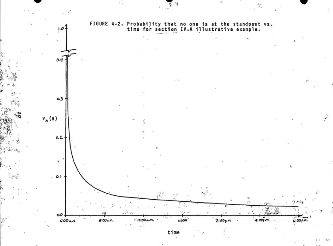
computer program using equation 4.2 was written to determinethis. The resulting curve for the illustrative example is shown
in Figure 4-2. Although v^(n) decreases with time, it remains
positive; there is always a possibility that no one is at the
standpost.
3. Line Lengths and Waiting Times
The PDF of the line length (which includes the person being
served) at the beginning of the nth interval can be used to determine the expected (i.e., average) line length, L(n), as
fol1ows :
L(n) =^j X V;(n)
,11J
(4.3)
For the illustrative example, the expected number of people in
line at the beginning of the second interval (6:03) is
L(2) = 0 X 0.368 + 1 X 0.368 + 2 x 0.184 + 3 X 0.061 + 4 X 0.015 + 5 x 0.003 +
6 X 0.001 1.00 person
.0--FIGURE 4-2. Probabi1ity that
time for section
no one is at the standpost vs
IV.A illustrative exam pie.
0.4
03 ͣ
-r>4
O
v„(n)
0.2-O. I
--O.0
UOOc
---h---
---1---/0.ͣOO<^,'»^,
---(---2:O0p,>vi.
Equation 4.3 includes the possibility that no one is in the
line (i.e., j = 0) to calculate the expected line length L(n).
However, when the line length is 0, no one is present to benefit
from the "shortness" of the line. The expected line length
experienced by customers must exclude time when the line is
empty. Therefore, it is of interest to know L'(n), the expected
line length given that the line is not empty (i.e., the expected
line length given that at least one person is at the standpost).
Atthebeginningofintervaln,
probability probability probability that that j persons = that the line x j persons are in
are in line is not empty line given that
the line is not empty
Referring to v-'(n) as the conditional probability that j people
are in line given that the line is not empty, the above equation
can be expressed in mathematical symbols as
V. (n) = (1 - v^(n)) x vj(n)
Solving for v.'(n) yields
J
v;(n) = Vj(n)/(1 - vjn))
(4.4)For the illustrative example. v,*(2) = 0.368/ v.'(2) = 0.291
V3'(2) = 0.097 v;(2) = 0.024 v; ( 2 ) = 0.005
1 - 0.368) = 0.582
Note that V:'(n) is always larger than VQ(n) by the constant
multiple 1/(1 - v^(n)). With the conditional probability of one
calculate L'(n), the expected line length given that the line is
not empty, as follows:
L'(n) = X j X v.;(n)
allj>0 J
Combining equations 4.4 and 4.5,
(4.5)
L'(n) = I j x v(n)/(l - v^(n))
cl(j>0
from which it follows that
(4.6)
L'(n) L(n)/(1 - V fn)) (4.7)
At the beginning of the second service period for the illustra¬
tive example,
L ' (2) = 1.00/(1 - 0.368)
= 1.58 pe rsons
which is substantially greater than L(2) = 1.00.
In addition to calculating the expected line length at the
beginning of any service interval, it is also possible to esti¬
mate the average amount of time persons arriving at the beginning
of the nth interval will have to wait to be served. W(n), which is the expected waiting time for the last person in line at the
beginning of the nth interval, is simply the product of the ex¬
pected number of service periods the person must spend at the
standpost, S(n), and the time required to serve each customer, .
W(n) includes both the time the customer spends in the queue
before beginning to be served and the time spent being served.
For a standpost with only one faucet, S(n) = L'(n). At the
beginning of the second service period for the illustrative
example,
W(n) = 1.58 persons x 3 minutes/person 4.74 minutes
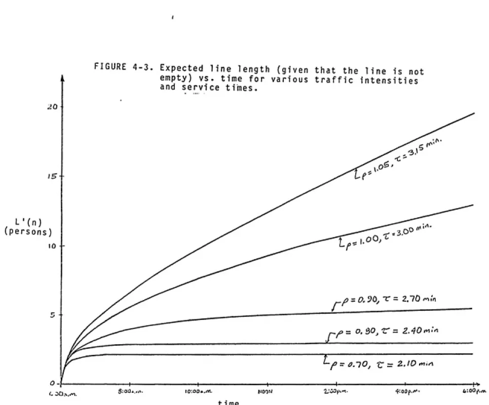
The "T = 3.00 minutes" curve in Figure 4-3 shows the in¬
crease in the expected line length L'(n) with time when the
expected arrival rate is 20 persons/hour, the service time is 3
minutes, and the discharge capacity is as determined by WHO
guidelines as shown on p. 11. For this curve the value of the
traffic intensity rho {p), which is the ratio of the expected
arrival rate A to the service rate capacity/^., is
p=X/^ = X/[l/r) = 20/hr / (1 / 3min)
1.00(The computer program used to determine the data points for the
curve is shown in Annex C.l.) Intuition might suggest that no
lengthy waiting lines would develop because the service rate
capacity is equal to the expected arrival rate, but such is not
the case. At 6:00 p.m., L'(n), the average line length given
that at least one person is at the standpost, is 13 persons.
With a service time of 3 minutes, this length corresponds to a
waiting time of 3x13 =39 minutes.An explanation of why L'(n) increases monotonically is as
fol1ows:
1. With T being the time since the standpost
began operating, the expected line lengthFIGURE 4-3
20
-IS -~
4--, L'(n)
(persons
10 —
Expected line length (given that the line is not
empty) vs. time for various traffic intensities
and service times.
oo, ^
^ = 0,'JO, -r = 2.70 ^.'n
£>- o. e>o, r" = -ii.'fO'vi.'i
arrivals during T minus the expected number
ofpeopleservedduringT.
L(T) - 'AT expected number served during T
2. The expected number served during T is equal
to the number of service intervals during T minus the expected number of service periods
during which no one is being served.
expected number =
served during T
expected number
l/Z - of service periods
during which no
one is served
3. Combining equations from steps 1 and 2 and noting from p. 12 that l/T is the service
ratecapacityy^-,
expected number
L (T) = XT - /xT + of service periods
during which no one is served
4. However on p.12 it was shown that X =/A, from
which it follows that
expected number L(T) = of service periods
duringwhich no
one i s served
5. As shown in Figure 4-2, the probability that
no one is in line is always greater than 0.
The expected number of service periods during
which no one is served during T thus increas¬ es with T. L(T) must therefore also
i n c r e a s e w i t h T.
6. Equation 4.7 expresses the relationship be¬ tween L'(T) and L(T). Since L'(T) is always
greater than L(T), L'(T) must also increase wi th T.
It is no coincidence that the traffic intensity /=> = 1.0
for the illustrative example. The WHO equation 3.1 sets the discharge capacity equal to the demand rate, with adjustments
guidelines assume that a service rate capacity equal to the
expected arrival rate is adequate, and do not consider the
possibility of lengthy lines shown by queuing theory.
Note that for the traffic intensity Z' > 1 the expected
arrival rate is greater than the service rate capacity, and for
^ <-1 the reverse is true. The traffic intensity therefore indi¬
cates the number of persons that are expected to arrive during
the time it takes to serve one person. It is of interest to
know the sensitivity of L'{n) to changes in p . Figure 4-3
illustrates this for /i) values of 1.05, 1.00, 0.90, 0.80, and
0.70. Note that forz? = 1.05 and with an expected arrival rate
A of 20 persons per hour, the service rate capacityyU. is 19.05
persons per hour, which is equivalent to a service period 'C
of 0.0525 hr per person, or 3.15 minutes. Such a situation
might exist for the illustrative example if time required to
position and remove the container from under the faucet were not
negligible, but were 0.15 minutes (9 seconds). For z? values less
than 1.0, the discharge capacity is increased to decrease the
service time '^, thereby increasing/^-. For example, forz? =
0.80, the discharge capacity is increased to reduce the service
period to 2.4 minutes, increasing the service rate capacity A to
25 per hour. Figure 4-3 shows that if a standpost is designed
such that service rate capacity is equal to or less than the
expected arrival rate (i.e., for P ^ 1.00) then L'(n) may be
undesireably long. When the service rate capacity significantly
exceeds the expected arrival rate (e.g.,/? = 0.80), results tend
of L'(n), is given by the following equation based on the litera¬
ture (Hillierand Lieberman, 1980):
L' = 1 + /5/[2(l -^)]
(4.9)This equation is applicable only when the service time does not
vary among customers, the standpost has only one faucet, the
expected arrival rate is constant, and the population is large
enough to be considered infinite. This equation can be used to
quickly determine the maximum expected line length (given that
the line is not empty) when it is known that L'(n) is essentially
at steady-state before the standpost closes or the arrivals
cease. Figure 4-3 shows that if/? is adequately less than 1.0,
steady-state is essentially reached very quickly, making equation
4.9 useful for such z) values. B. Variable Arrival Rates
Accounting for an expected arrival rate that changes over
time is quite straightforward. X is assumed to be constant
for any particular service interval but is allowed to vary from
one interval to the next. The variation is therefore approxi¬
mated by a discrete function, which requires the application of
equation 4.1 at each step. The model remains essentially the
same as that presented in the previous section, except that new p
values must be calculated for each service period having a
different^. This recalculation is necessary because p^^^ is a
functionofX.
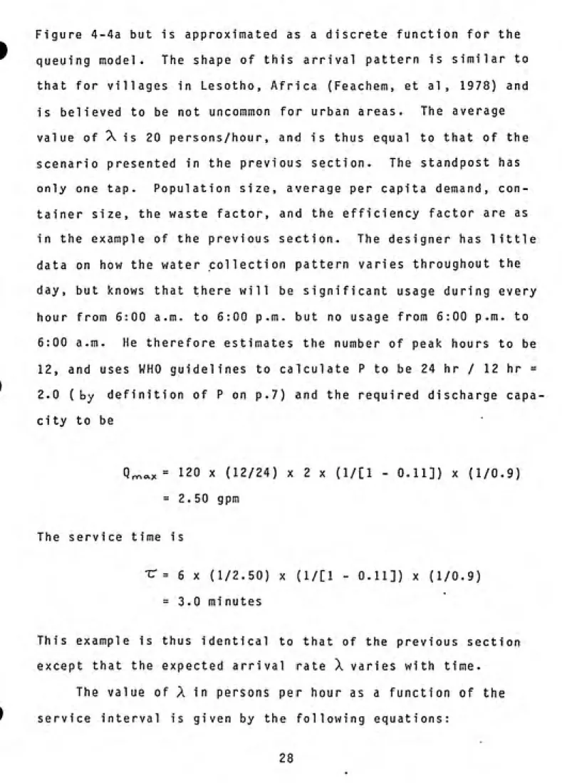
To illustrate the application of queuing theory to a
time-varying expected arrival rate, X is assumed to vary as shown in
Figure 4-4a but is approximated as a discrete function for the
queuing model. The shape of this arrival pattern is similar to
that for villages in Lesotho, Africa (Feachem, et al, 1978) and
is believed to be not uncommon for urban areas. The averagevalue of 'X is 20 persons/hour, and is thus equal to that of the
scenario presented in the previous section. The standpost has
only one tap. Population size, average per capita demand, con¬
tainer size, the waste factor, and the efficiency factor are as
in the example of the previous section. The designer has little
data on how the water collection pattern varies throughout the
day, but knows that there will be significant usage during every
hour from 6:00 a.m. to 5:00 p.m. but no usage from 6:00 p.m. to
6:00 a.m. He therefore estimates the number of peak hours to be
12, and uses WHO guidelines to calculate P to be 24 hr / 12 hr =
2.0 (by definition of P on p.7) and the required discharge capa¬
city to be
Q^^^ = 120 X (12/24) X 2 x (1/Cl - 0.11]) x (1/0.9)
= 2.50 gpm The serVice time is
-^ = 6 x (1/2.50) x (1/[1 - 0.11]) X (1/0.9)
= 3 . 0 m i n u t e s
This example is thus identical to that of the previous section
except that the expected arrival rate X varies with time.
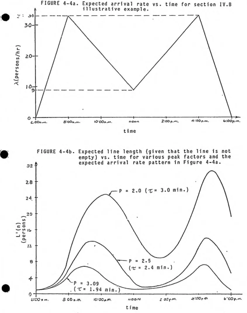
The value of A in persons per hour as a function of the
FIGURE 4-4a. Expected arrival rate vs. time for section IV.B illustrative example.
30 —
o <v
C.COo r.i. 8-OOa.,t\ lO COa.^ 2-00 p.m. 4 ͣ OOp.rM. fc:OOp./>i.
time
FIGURE 4-4b. Expected line length (given that the line is not
empty) vs. time for various peak factors and the
expected arrival rate pattern in Figure 4-4a
9 4 m i n.)
^.ͣ OO 1^1
3 00 o ix^ h 'CO p, ."
X(n ) = 34 X n/40
A(n) = 46.5 X (148.8 - n)/148.8
X(n) = 34 X (n - 91.2)/108.8
A(n) = 34 X (240 - n)/40
for 0 :^ n ^ 40 (4.10) or 6:00 a.m. to
8:00a.m.
for 40 < n < 120 (4.11)
or 8:00 a.m. to
noon
for 120 < n < 200 (4.12) or noon to 4:00 p.m.
for 200 £ n < 240 (4. 13)
or 4:00 p.m. to
6:00p.m.
To determine, for example, the probability that the line at
the standpost is empty at the beginning of the second service
period, equation 4.2 is applied as in the constant expected
arri-ratecasetoobtain
Vg(2) = Vo (1) X Po(from 6:00 a.m. to 6:03 a.m.) +
v,(l) X p^(from 6:00 a.m. to 6:03 a.m.)
From equation 4.10, the A value for determining p^{from 6:00
a.m.to6:03a.m.)is
A (1) = 34 X 1/40 - 0.85 per hour
and , by equati on 4.1,
p^(from 6:00 a.m. to 6:03 a.m.)
0 -(0.85/hr X 0.05hr)
(0.85/hr X O.OShr) e / 0!
=0.9 58Given that v^(l) = 1.0 and v,(l) = 0.0,
v„(2) = 1.0 X 0.958 + 0.0 x 0.95!
Thus, the procedure for determining probability values v-(n),
line lengths given that someone is at the standpost, and waiting
times, is exactly the same as when the expected arrival rate is
constant, except thatX(n) must be calculated for each service
period.
The resulting L'(n) values are shown by the P = 2.0 curve in
Figure 4-4b. (The curve was calculated by the computer program in
Annex C.4,) L'(n) reaches much greater values than shown by the
p - 1.00 curve in Figure 4-3, even though the average^ value
for the time-varying case is also 1.0. For example, at about
4:50 p.m. L'(n) for the time-varying case is 31 persons,
corresponding to an expected waiting time W(n) of 31 x 3 = 93
minutes, which is quite long. The L'(n) value from thez3 = 1.00 curve in Figure 4-3 at 4:50 is 12, corresponding to an
expected waiting time of 36 minutes. The time variation in the
expected arrival rate is obviously an important consideration in
standpostdesign.The designer may suspect that usage during the 12-hour
period from 5:00 a.m. to 6:00 p.m. varies significantly, and
although he may not know the extent of the variation, he may wish
to chose a more conservative peak factor of 2.5 to account forthe variation. The required discharge capacity by WHO guide¬
line s w o u 1 d b eQ^,, = 120 X (12/24) x 2.5 x (1/[1 - 0.11]) x (1/0.9)
= 18 7 gal 1 ons/day = 3.1 gpm
The service time would be
^ =6 X (1/3.1) x(l/Cl- 0.11]) X (1/0.9)
= 2.4 mi nutesThe computer program used to determine L'(n) for P = 2.0 was
modified to determine L'(n) for P = 2.5. The resulting curve is
shown in Figure 4-4b. L'(n) reaches its maximum value of 14
persons at 4:30. The corresponding expected waiting time is 14 x
2.4 = 34 minutes, which is still rather long.
The designer may perceive that a thorough investigation of
the water collection pattern is warranted before designing the
standpost. If he collects data to estimate the usage during
every hour between 6:00 a.m. and 6:00 p.m., he would find that
peak hourly usage occurs during the hour from 8:00 a.m. to 9:00
a.m. and the hour from 3:00 p.m. to 4:00 p.m. He would find that
the average number of arrivals during either of these hours is
A = (34 persons/hr + 27.75 persons/hr) / 2 = 30.9 persons/hr
'—-A at 8:00 a.m. ^—A at 9:00 a.m.
from e-3n. 4.10 'porii eon.A-.li
The peak factor P would then be simply the ratio of this peak
hourly expected arrival rate and the average expected arrival
rate over the 24-hour period, or 30.9/10 = 3.09. The required
discharge capacity by WHO guidelines would be 3.86 gpm. The
service time would be 1.94 minutes. Computer program results,
which are shown in the P = 3.09 curve in Figure 4-4b, show that
L'(n) would reach its maximum value of 6.65 persons at 4:18 p.m.
The corresponding expected waiting time is 6.65 x 1.94 = 12.9
The peak factor of 2.0 provides a service rate capacity of
Jbi- \IX- 1 person/3minutes = 20 persons/hour. This rate is equal to the expected arrival rate averaged over the peak period
of 12 hours. The average value of ^ over this 12-hour period
is therefore 1.0. The peak factor of 2.5 provides a service rate
capacity of 25 persons/hour, which is equal to the expected
arrival rate averaged over the peak period of 4 hours extending from 6:55 a.m. to 10:55 a.m. (or from 1:05 p.m. to 5:05 p.m. for
the later of the twin peaks). When P = 2.5, the average p
value over this 4-hour period is 1.0. The peak factor of 3.09
provides a service rate capacity of 30.9 persons/hour and an
average ^ value of 1.0 over the 1.0-hour period extending from
8:00 a.m. to 9:00 a.m. (or from 4:00 p.m. to 5:00 p.m.).
The WHO guidelines state that the peak period is the time
during which "the standpost is used more intensively than during
the rest of the day", that it typically lasts between 4 and 12
hours, and that there is a time-varying water demand pattern
during the peak period. Because the demand varies with time
during the peak period, the peak demand estimate will tend to increase as the length of time selected for the peak decreases.
This is clearly shown by the difference in P factors for the
above examples. Peak periods of 12 hours, 4 hours, and 1 hour correspond to peak factors of 2.0, 2.5, and 3.09,
respectively. The guidelines do not indicate how to select the length of the peak period, but indicate 4 to 12 hours to be the range of typical lengths. However, for the above example, using
peak period of only 1 hour yields reasonable results (a maximum
L'(n) value of 6.65 persons) but even this line length might be
considered unacceptable if service times are not short. Forexample, if the service time is 5 minutes this length corresponds
to an expected waiting time of 6.65 x 5 - 33 minutes.The guidelines also state that the peak factor is typically
in the range of 2 to 4. When the designer selects 3.1 for the conditions of this example, the maximum expected waiting time is
reasonable. However, in some cases even a peak factor of P = 4 will not provide adequate discharge capacities. Assume, for
example, that the arrival pattern is identical to that of Figure 4-4a except that no arrivals occur after noon. People rely on
another source in the afternoon because the standpost is closed.
The daily demand from the standpost is thus reduced from 1440
gallons/day to 720 gallons/day. The average hourly demand from
6:00 a.m. to noon would be 720/6 = 120 gallons/hour, and the av¬
erage hourly demand over the day would be 30 gallons/hour. If a
peak factor of P = 120/30 = 4 is used, the resulting discharge
capacitywouldbe
Qmax = 120 x (6/24) X 4 X (1/[1 - 0.11]) x (1/0.9)
= 150 gal 1ons/day = 2 . 5 g p m
The service time would be
-r = 6 X (1/2.5) X (1/[1 - 0.11]) x (1/0.9)
= 3 . 0 mi nutes
for the example resulting in the P = 2.0 curve in Figure 4-4b.
The L'(n) values would thus equal those shown by the P = 2.0
curve from 6:00 a.m. to noon. The maximum L'(n) value is 25
persons. The corresponding expected waiting time is 25 x 3 = 75
minutes, which is very long.
C . M u 1 t i p 1 e F a u c e t s
Incorporating multiple faucets into the large-population
model is accomplished by recognizing that the maximum number of
departures which can occur during a service interval is no longer
1 as in the single faucet case, but is equal to the number of
faucets. If, for example, there are two faucets, then equation
4.2mustbemodifiedas follows:
v;(n + 1) = Z (v- (n) x p JT))
1=0
(4.14)
wherek=j if i=Oorl k = j - i + 2 if i > 1
The derivation of this equation is analogous to that
starting on p. 15 for the single faucet case. For example, the
mutually exclusive events which can account for one person at the standpost at the beginning of the second service interval with
two faucets is as follows, which can be compared with its counterpart on p. 17 for a single faucet.
V,(2) = v^(l) x p,(T) + V,(1) X p,(r) +
v^(l) X p, (TT) + V3(l) X p^(-r)
Equation 4.2 can also be modified for three or more faucets
by taking into account that the maximum number of people served
Any even number of persons at a two-faucet standpost results
in a number of service periods equal to one-half the number of
persons. Three or any higher odd number of persons at a
standpost with two faucets results in a number of service periods
equal to one-half the difference between that number and 1.
S(n), the expected number of service periods spent in line, is as follows for a two-faucet standpost.
S(n) = 1 x v;(n)
+ 0.5 x 2 x v^(n)
+ 0.5x4xv^(n)
0.5 X (3 0.5 X (5
1) 1)
X vi(n)
(n)
X V
(4.15)
The advantage of using S(n) over L'(n) is that it gives a better
indication of how long a person is expected to wait when there is
more than one faucet at the standpost. The expected waiting time
is determined simply by multiplying S(n) by tr , the time required
to serve one person. When the standpost has only one tap, S(n)
= L'(n), but when there is more than one faucet, S(n) < L'(n).
To illustrate the queuing model for a two-faucet standpost,
assume that the arrival pattern is as shown in Figure 4.4a and
that the scenario is identical to that of the previous section.
A peak period of 1 hour is used and, as shown in the previous
section, this result in a peak factor P = 3.09 and a WHO required discharge capacity of 3.85 gpm. The discharge capacity per
faucet is 3.86/2 = 1.93 gpm. The service time is
-^ = 6 X ( 2 / 3 . 86 ) X (1 / [ 1 - 0 .11 ] ) X (1 /O . 9 ) = 3.9 mi nutes
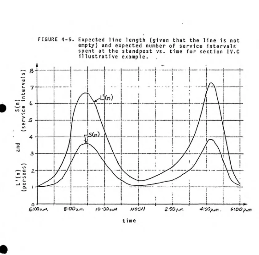
C.6. The results are shown in Figure 4-5.
The maximum values of the expected line length (given that
at least one person is at the standpost) and the expected number of service periods spent at the standpost are 7.2 and 3.9,
respectively. The corresponding maximum expected waiting time is 3.9 X 3.9 - 15.2 minutes. In the previous section the single-faucet example with a peak factor of 3-09 resulted in a maximum
expected waiting time of 12.9 minutes, which is a bit less than
that of this two-faucet example. One might be surprised by this
difference because the standpost discharge capacities are equal in these two examples. The service time at the two-faucet
stand-post is twice as great as at the single-faucet standstand-post because
the flowrate through each of the faucets is half as great. Al¬
though the service time is twice as great, one would expect the
number of service periods spent at the standpost to be halved
because of the extra faucet, and that the waiting times for these two examples would be equal. However, when only one person is at the standpost the availability of a second faucet does not reduce
that person's waiting time. Similarly, when some higher odd number of persons are in line, the number of service intervals required to serve all of them is the same as if one additional customer were in line. In general, if two standposts have equal discharge capacities, the one with the greater number of faucets will have slightly longerwaiting times.
Figure 4-6 applies to constant expected arrival rates. The
Figure shows S, the steady-state expected number of service
intervals spent at the standpost vs. the traffic intensity Z? (the
FIGURE 4-5. Expected line length (given that the line is not
empty) and expected number of service intervals
spent at the standpost vs. time for section IV.C illustrative example.
tJOCfi 2-0D>>.M
Qj'QOa.yt
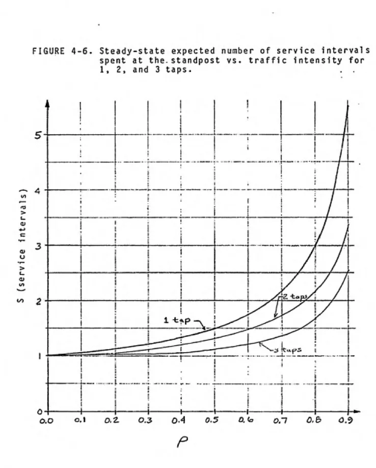
FIGURE 4-6. Steady-state expected number of service intervals
spent at thestandpost vs. traffic intensity for
1 , 2, and 3 taps. . ,
n3
rate capacity cm, where c is the number of taps and ^ is the
service rate capacity per tap) for 1, 2, and 3 faucets. For the
single-faucet curve, values were obtained by use of equation 4.9,
with S = L'. For the multiple-faucet curves, values were ob¬
tained by the computer programs shown in Annexes C.2 and C.3.
These computer programs do not actually calculate true
steady-state values, but calculate values for 400 service periods, which
is a long enough time for steady-state to be essentially reached
when/? = 0.9. Values for p close to but less than 1.0 are not
included in Figure 4-6 because of the lengthy time required to
reachnearsteady-state.
Figure 4-6 shows that at a given^ value, S decreases as the
number of faucets increases. For example, at z? = 0.8, S = 3.00 for one faucet and S = 1.66 for three faucets. However, as dis¬
cussed previously, for a given standpost discharge capacity the
steady-state expected waiting time W increases as the number of
faucets decreases. Assume for example that the standpost dis¬
charge capacity is 4.00 gpm, making the service time to be 2.00
minutes when there is one faucet. For three faucets the flow per faucet would be 1.33 gpm, making the service time to be 6.00 minutes. The resulting steady-state expected waiting time W at
p= 0.8 would be 3.00 x 2.00 = 6.00 minutes for one faucet, and
1.66 x 6.00 = 9.96 minutes for three faucets.
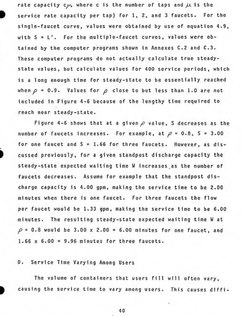
D. Service Time Varying Among Users
The volume of containers that users fill will often vary,
diffi-culty in applying the Poisson equation because the value of -XT used in the equation is variable. This difficulty can be over¬
come by selecting probability distributions which are in a form which lend themselves to the numerical modeling of queues. How¬
ever, such models are not presented in this paper for the follow-in g r e a s o n s :
1. For a constant expected arrival rate, the steady-state line length at an adequately designed standpost will be reached fairly quickly. Figure 4-3 shows how soon steady-state is reached when P (the traffic intensity, which is the ratio of the expected arrival rate to the service rate capacity) is adequately low. Reaching steady-state requires more time
when p is higher. Although steady-state equations may not
accurately calculate line lengths at underdesigned
stand-posts (because^ is too high and the standpost may close or
arrivals may stop before steady-state is reached), they can be used to adequately design standposts, making numerical modeling unnecessary when the expected arrival rate is con¬stant.
2. Koopman (1972) has shown that for time-varying expected
arrival rates, the variation in service time among users does not seem to have a substantial impact on expected line lengths. Thus, when the expected arrival rate var¬ ies, the service time among users may be assumed constant
and the queuing model of the previous section may be appli ed .
The following equation, which can be obtained from queuing
theory texts (e.g., Hillier and Liebermann, 1980), determines L',
the steady-state expected line length given that the line is not empty. The equation is applicable for any service time proba¬
bility distribution, but the expected arrival rate must be con¬
stant, the standpost must have only one faucet, and the popula¬ tion must be large enough to be considered infinite.
L' == I + (-/'4 + /^)/[2^(l -^)] (4.16)
Equation 4.16 is applicable only if n (the traffic intensi¬
ty) is less than 1. If p is equal to or greater than 1, then
steady-state is never reached and equation 4.16 is meaningless.
Also, the equation should only be used if it is known that
steady-state is reached before arrivals cease or the standpost closes.
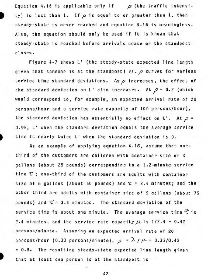
Figure 4-7 shows L' (the steady-state expected line length
given that someone is at the standpost) vs. p curves for various
service time standard deviations. Asz? increases, the effect of
the standard deviation on L' also increases. At/?= 0.2 (which
would correspond to, for example, an expected arrival rate of 20
persons/hour and a service rate capacity of 100 persons/hour),
the standard deviation has essentially no effect on L'. kt p =
0.95, L' when the standard deviation equals the average service time is nearly twice L' when the standard deviation is 0.
As an example of applying equation 4.16, assume that
one-third of the customers are children with container size of 3
gallons (about 25 pounds) corresponding to a 1.2-minute service
time T ; one-third of the customers are adults with containersize of 6 gallons (about 50 pounds) and T = 2.4 minutes; and the
other third are adults with container size of 9 gallons (about 75
pounds) and ir= 3.6 minutes. The standard deviation of the
service time is about one minute. The average service time 'V is
2.4 minutes, and the service rate capacity^ is 1/2.4 = 0.42
persons/minute. Assuming an expected arrival rate of 20
persons/hour (0.33 persons/minute), p = ^ Ip- = 0.33/0.42
/J>-'
{y.
(persons
FIGURE 4-7. Steady-state expected line length (given that
the line is not empty) vs. traffic intensity
for 1 tap and various service time standard
deviations.
L' - 1 + (0.333^x 0.98^+ 0.8^)/C2 x 0.8 x (1 - 0.8)]
= 3.33 pe rsons
If the standard deviation were 0, L' would be L' = 1 + 0.8"/(2 x 0.8 x [1 - 0.8])
= 3.00 pe rsons
The increase in L' due to the variation is service time is thus
100% x (3.33 - 3.00)/3.33 = 11% for this example.
By multiplying equation 4.16 by T(the average service
time) and using /^ =\iM- = '^'^ , the steady-state expected waiting
time W for a single-faucet standpost and constant expected
arrival rate is as follows:
W = ^+A( crj" + r^)/(2>^[l -Xx]) (4.17)
For the above example, equation 4.17 shows that the steady-state
expected waiting time W when the service time standard deviation cCis 0 is 7.20 minutes, and 8.00 minutes when the standard devi¬
ation is a minute. The increase in W due to the standard devia¬
tion is (8.00 - 7.20)/7.20 x 100% = 11%, which is of course the
same percent increase the standard deviation causes in L'.
Based on a telephone operator staffing study done by Sze
(1984), the percent increase in the steady-state expected waiting
time W that the service time variation causes when there are
multiple faucets is the same as the percent increase when there
is a single faucet, assuming that the average of the varying
two taps. Based on Figure 4-6 W = 2.2 x 2.4 = 5.3 minutes.
If the service time standard deviation were increased to 1.0
minute, as in the previous example, then the steady-state ex¬
pected waiting time W would be increased by 11%. The new value
ofWwouldbel.llx5.3=5.9minutes.
Figures 4-8 and 4-9 show for the effect that the service time
standard deviation cX^ has on S (the steady-state expected number
of service periods customers spend at the standpost) for two and
three taps, respectively. The curves for cXj-> 0 were determined
with the knowledge that S is directly proportional to W, and that
the percent increase in S due to o^is therefore the same for mul¬
tiple faucets as it is for one faucet.
Understanding why the service time variation causes W to
increase may prove useful. While customers having short service times are served, the service rate capacity is in effect in¬
creased, thereby decreasing the jO value during that service time.
While customers having long service times are served, the oppo¬
site occurs. Both long and short service times effectively
change z> temporarily. However, the relationship between W and /? is concave-up (i.e., as z? increases, the W vs. z? curve becomes
steeper). Therefore, longer service times cause a greater in¬
crease in W than do the shorter service times cause a decrease in W. The net effect is that W is greater when the service time varies among users than when service time is constant amongFIGURE 4-8. Steady-state expected number of service intervals
spent at the standpost vs. traffic intensity for 2 taps and various service time standard
deviations.
> CD
o >
FIGURE 4-9. Steady-state expected number of service intervals
spent at the standpost vs. traffic intensity for
3 taps and various service
deviations.
time standard
> +->
cz
U > u.
00
OO
i:
A
-- i
ͣ
i
I ! t
j\
i 1 . I ' :
i ^ [
1«
ͣ
o .
i
/ J
!
//
-9 .
l;"X/^
i
/ y...;
—=
=:^^^^
1---._ J
tfl^=6 1
1 ͣi
(.---1 1---1
i
1
0 ͣ
ͣ
\ 1
---^---;---j—^—
---0.0 0.1 0.2. 0.3 0.4 0.5 0.(c o.l 0.^ 0.9
Chapter V
SMALL-POPULATION MODEL
The large-population models of Chapter IV are based on the assumption that the population is large enough to be considered
infinite. This assumption allows for model simplicity and flexi¬
bility. Populations should therefore be assumed infinite when¬
ever they are large enough for the assumption not to cause signi¬
ficant inaccuracies. In this chapter a small-population model
(i.e., a model that does not assume the population is infinite)
will be derived. In Chapter VI its results will be compared with
the results of the model presented in section IV.A. Minimum population sizes which can be assumed to be infinite without
causing serious inaccuracies will thus be determined. The same
four assumptions listed on page 10 for the large-population model
are also assumed for the smal1-population model so that any
difference in results may be attributed strictly to the
limita-tionofpopulationsize.
The small-population model is similar to the large-popula¬
tion model in that expected queue lengths are calculated at times
which are interger multiples of the service period, i.e., expect¬
ed line lengths are calculated at the beginning of the second
service period, the beginning of the third service period, etc. However, the derivation of the small population model is more
complex because the number of arrivals during any particular
service period affects the PDF of the number of arrivals during
other service periods. The reason for this is that the number of
arrivals that have occured may be a significant portion of the
arriv-als. The model derivation consists of the following steps:
1. Determining the PDF for the number of arrivals at the
standpost during any service period.
2. Using the PDF in step 1 to develop the PDF for sequences
of arrivals over a series of consecutive service periods.
(One of the probabilities expressed by this PDF would
be, for example, the probability that 2 arrivals occur in the first service period, 0 arrivals occur in the second
service period, and 4 arrivals occur in the third service period.)
3. Using the PDF determined in step 2 to calculate expected
line lengths and waiting times.
These steps are discussed below. Assume that a
single-faucet standpost serves a population of 20 customers. All of
the customers arrive at the standpost between 6:00 a.m. and 7:00
a.m.; employment away from home, school, etc., make other times
inconvenient. The size of containers is assumed to be 6 gallons
and the discharge capacity is 2.5 gpm. The waste factor w is
0.11 and the efficiency factor f is 0.9. The resulting service
time TT is, by equation 3.2,
r = 6 K f ] /2.5 ) X (1/[1 - 0.11]) x (1/0.9) = 3.0 minutes
The scenario is therefore identical to that of section IV.A except that the population is limited to 20 and arrivals occur only between 6:00 a.m. and 7:00 a.m.
1. Probability Density Function of the Number of Arrivals
DuringaServicePeriod
Because the expected arrival rate is assumed not to vary with
time, each member is just as likely to arrive between 6:00 a.m. and 6:03 a.m. as between, say, 6:30 a.m. and 6:33 a.m. The
probability that a particular customer (i.e., an arbitrarily
chosen customer out of the population of 20) arrives during some time period of length Twithin T is simply t^/T. If T is the
1-hour period from 6:00 a.m. to 7:00 a.m. and ^ is 3 minutes
(0.05hr), then this probability is 0.05hr/1.0hr = 0.05. The probability that two particular customers arrive during a time period of length 1Z is [XIT) x ('C7 T). The customers act indepen¬ dently of each other and their probabilities of arriving during a period of length Tare therefore multiplied to determine the joint
probability that both arrive during the period of length X . In
general, the probability that k particular customers arrive dur-ing a time period of length IT" is (T/T) .
Similarly, if the population is N, the probability that
N - k particular customers arrive outside of a time period of
H -K
length X but still within time period T is ([T -TJ/T)
The probability that k particular customers arrive during a
time period of length "X. and N - k particular customers arrive
0 u t s i d e 0 f IT (i . e . , d u r i n g T - 'C ) i s
(r/T)*" X ([T --r]/T)'^"*'
The probability that any k customers arrive during a period
of length '"J' and ^r\)i N - k customers arrive during T -fis an
integer multiple of the above product. The integer is the number
N, which is the permutation
N!/(k![N - k]! )
Therefore, defining r ^^^ (T) as the probability that k
customers arrive during a period of lengths;,
r^ir) = (N!/(k![N - k]!))(Tr/T)'^([T -'i:]/T)'^~'' (5.1)
Equation 5.1 is a form of the binomial distribution. For exam¬
ple, the probability that 2 customers arrive between 6:00 a.m.
and6:03a.m. isr^(0.05hr) = (20 !/2 ! 18 ! ) (0 . 05hr/1.Ohr)^(0.95hr/1.Ohr)^°'
=0.189
Because the entire population of 20 arrives in a 1-hour period and the expected arrival rate does not vary with time, the
expected arrival rate is 20/hr. Table 5-1 compares the proba¬
bilities when applying the Poisson equation (equation 4.1) and
the binomial equation (equation 5.1) over a 0.05hr period when
the expected arrival rateX= 20 persons/hr. The Poisson equation
assumes the population is infinite, whereas the binomial equation
assumes a population size of N, which in this example is 20. It
is well known that as N increases, the results of the binomial
equation approach those of the Poisson equation. Table 5-1 shows
that when the number of arrivals k is equal to 1, which is the
expected number of arrivals per service period, rj^(0.05hr) >
p (O.OBhr). That is, the probability of 1 arrival during a time
period of length 'C is greater when the population is 20 than
true when the number of arrivals k = 2. However, in general,
r ('t') is less than P^(T') for values of k different from the
expected number of arrivals per service period.
TABLE 4-1
Comparison of Binomial (N - 20) and Poisson (N
Equation Results for T = 0.05 hr
cx:> )
r^(0.05hr) pjO.OShr)
0 0.3 58 0.368
1 0.377 0.368
2 0,189 0.184
3 0.060 0.061
4 0.013 0.015
5 0.002 0.003
6 0.000 0.001
7 0.000 0.000
20 0.000 0.000
2. Probability Density Function for Sequences of Arrivals
During a Series of Consecutive Service Periods
With known PDF of arrivals during the first service period
and given that no one is in line at 6:00 a.m., equation 4.2 can be used to determine the PDF for the number in line at the be¬
ginning of the second service period. For this purpose, the
r (T) values in Table 5-1 are used in place of p^(t) because the
population is 20 instead of infinite. The PDF can then be used to calculate the expected line length at the beginning of thesecond service period.
Calculating the PDF and expected line length at the begin¬
ning of the third service period is more difficult due to thefact that arrival probabilities during the second service period
occur during the first period then the probability of three ar¬
rivals in the second period is different than if only one arriv¬
al had occured during the first period. It is therefore neces¬sary to determine the probability of sequences of arrivals.
To determine the probabilities of sequences of arrivals, let
the variables k, and k^ represent the number of arrivals in the
first and second periods, respectively. The probability of kj.arrivals during the second period given that k, arrivals have
already occured in the first period can be determined by equation
5.1, but with the population reduced to N - kj and T reduced to
T -T. Thi s pr obabi 1 i ty i s
([N-k,]!/(k![N - k, - kj!))(r/[T -'U]f^([T -r-r]/[T -V}{'^'~'^'
In the above expression, the probability of k2 arrivals in
the second interval is conditional on the probability of k,arriv¬
als in the first interval. The product of the two probabilities
is therefore equal to the joint probability that k, arrivals
occur in the first interval and k^ arrivals occur in the second.
Multiplying the two probabilities yields
\^^2., ,N -k,-k.
r , (T) = [N!/(k,!ki (N - k, - k)!)](r/T)' ^((T-2r)/Tj ' ^ (5.2)
')it-Similarly, the joint probability of k, arrivals in the first
period, k^^ arrivals during the second period, and k^ arrivals
in the third period is