Advancements in Methodologies and Theories Regarding Model
Membrane Environments by Total Internal Reflection with
Fluorescence Correlation Spectroscopy
by Jamie Kay Pero
A dissertation submitted to the faculty of the University of North Carolina at Chapel Hill in partial fulfillment of the requirements for the degree of Doctor of Philosophy in the Department of Chemistry.
Chapel Hill 2006
Approved by:
ABSTRACT
Jamie Kay Pero: Advancements in Methodologies and Theories Regarding Model Membrane Environments by Total Internal Reflection with
Fluorescence Correlation Spectroscopy (Under the Direction of Nancy L. Thompson)
Total internal reflection with fluorescence correlation spectroscopy (TIR-FCS) was utilized to determine the diffusion coefficient of nine fluorescently labeled antibodies, antibody fragments, and antibody complexes approximately 85 nm from a planar membrane. The diffusion coefficient decreased with increasing molecular size over what would be expected from the Stokes-Einstein Equation. Theory was derived specific to use with TIR-FCS to describe spatially dependent diffusion near membranes. The decreased diffusion is likely due to increased frictional coefficients when molecules are in close proximity to membranes. This described spatially dependent diffusion could be one contributor to the nonideality observed in ligand-receptor kinetics at membranes.
than the primary bilayer. The stacked bilayer system will have application in multilayer systems and as a cushioning system. Other applications are likely forthcoming.
To Mom and Dad…..
Thanks for the love, support, financial aid and occasional harassment (Dad).
And to Ellie Mae……
ACKNOWLEDGEMENTS
As I grow nearer to completing my thesis, I find myself growing more reflective and searching for some level of fruition for this chapter of my life. I realize at this time that I cannot separate the work and the role of graduate student from who I inherently am. I have come to a type of symbiotic relationship between me and my research. Consequently, those who I am thanking now, I am thanking for molding me into who I am today.
I would like to begin with my advisor. When I look back to four years ago I am embarrassed at how naïve and rough I was. I had no clue what I was going to learn personally and professionally in the next part of my life. It takes special people to do that year after year, individual by individual. So, Nancy, thank you for allowing me to screw up and grow up.
And mom and dad….you know me better than any other people on this earth. You have seen the full range of my personality. You know the worst and the best of me. And yet you are still there for me, encouraging me on and seeing talent that I don’t believe is there. From spelling bees to drama play and on to thesis’……you’ve always thought I could move mountains. I appreciate that unwavering faith in me and most of all the deep love. This PhD is as much yours as it is mine. I love you both.
To my brothers…..Occasionally you have thought I was nuts and high-spirited. Other times you’ve thought I was mischievous, but there you were riling me up and getting me going or lending a sympathetic ear. I love you all for different reasons. Jeremy, I admire your patience, heart, and awareness of that greater humanity that so few possess. Jeff, I love your competitive spirit, belief in yourself, and conquering attitude. Jordan, I am moved by your sensitivity, your HARD work, and the depth of your soul.
have done. Please look at my accomplishments as a reflection of what your sacrifice has brought. I love you all!!!
To my friends……There are so many of you and so many reasons to thank you so I am going to keep this brief but know how much you have helped me to get to this point. If you hadn’t talked me through so much of this, I don’t know that I would be here. Thank you to Emily and Kristin for dancing in lab, yogurt runs, the spice girls, and our “infamous” lab talks. Thank you to Patricia for taking me in my first year and giving me an instant group of friends. I truly appreciate our friendship. Here’s to Italy!!! Thank you to Erin, Melissa, Katie, and Ginger for the occasional house fire and dinner party but especially for our “group counseling sessions.” Thank you to Jenn for not seeing me as a nuisance our first year and always being willing to teach me things. Your friendship means a lot. Thank you also to Caia, Christie, Kalpana, Domenick, Becky, and everyone else. Chapel Hill would not have been the same without our adventures and our support system!!!
And finally thank you to Justin. I met you late in my graduate career. But you more than anyone else know what was put into this thesis. You saw me cry, worry, and wear myself out. And you still like me! Thank you for housing me, caring about me, and being willing to take a leap of faith. Please know that I see the deep goodness in you and your spirit. I am completely aware of how much I need you. Thank you also to Susan and Scooter Parker for allowing me to hibernate in their basement and providing food and computer paper during the writing of this thesis!
TABLE OF CONTENTS
LIST OF TABLES... xi
LIST OF FIGURES ... xii
LIST OF ABBREVIATIONS... xiv
LIST OF SYMBOLS ... xvi
Chapter 1 Introduction ...1
Chapter 2 Size Dependence of Protein Diffusion Very Close to Membrane Surfaces: Measurement by Total Internal Reflection with Fluorescence Correlation Spectroscopy...13
2.1 Abstract ...13
2.2 Introduction...13
2.3 Theoretical Background...17
2.3.1 Apparatus ...17
2.3.2 Fluorescence Fluctuation Autocorrelation Function G( )...19
2.3.3 Magnitude of the Fluorescence Fluctuation Autocorrelation Function ...19
2.3.4 Shape of the Fluorescence Fluctuation Autocorrelation Function for Spatially Independent Diffusion ...20
2.3.5 Spatially Dependent Diffusion Coefficients ...21
2.4.1 Antibody Preparation...26
2.4.2 Phospholipid Vesicles...28
2.4.3 Substrate-Supported Phospholipid Bilayers ...28
2.4.4 Fluorescence Microscopy ...29
2.4.5 Data Analysis ...30
2.5 Results...32
2.6 Discussion...39
Chapter 3 Stacked Phospholipid Bilayers on Planar Supports ...42
3.1 Abstract ...42
3.2 Introduction...42
3.3 Theoretical Background...46
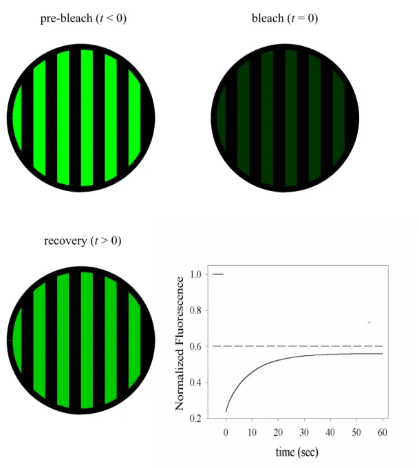
3.3.1 Fluorescence Pattern Photobleaching Recovery (FPPR)... 46
3.3.2 F-Statistics...47
3.3.3 Order Parameter Measurements...49
3.3.4 Atomic Force Microscopy ...50
3.4 Materials and Methods...53
3.4.1 Avidin and Soluble Biotin ...53
3.4.2 Sonicated Vesicles ...54
3.4.3 Slide Cleaning...55
3.4.4 Intensity Measurement and FPPR Measurement Slide Preparation ...55
3.4.5 Order Parameter Measurement Slide Preparation...56
3.4.6 Atomic Force Microscopy Slide Preparation...56
3.4.8 FPPR and Intensity Measurements ...57
3.4.9 Order Parameter Measurements...57
3.4.10 Atomic Force Microscopy ...58
3.5 Results...58
3.5.1 Control Measurements ...58
3.5.2 Intensity Measurements ...59
3.5.3 Specificity of NeutrAvidin Binding to Biotinylated Lipids...61
3.5.4 Mobility of FNA bound to Biotinylated Lipids ...63
3.5.5 FPPR Measurements...63
3.5.6 Order Parameter Measurements...66
3.5.7 AFM Measurements...69
3.6 Discussion...72
Chapter 4 High Refractive Index Substrates to Generate Very Small Evanescent Wave Depths...75
4.1 Abstract ...75
4.2 Introduction...76
4.3 Theoretical Background...82
4.3.1 TIR-FCS...82
4.4 Materials and Methods...82
4.4.1 Substrate Preparation ...82
4.4.2 Antibody Preparation...82
4.4.6 TIR-FCS Experiments ...84
4.4.7 Data Analysis ...85
4.5 Results...85
4.5.1 Fluorescence Imaging ...85
4.5.2 Native Luminescence of TiO2and SrTiO3...87
4.5.3 Fluorescent Antibody Experiments...90
4.5.4 TIR-FCS...92
4.5.5 Quenching Phenomenon ...94
4.6 Discussion...94
Chapter 5 Summary and Future Directions ...98
APPENDIX: TIR-FCS AUTOCORRELATION FUNCTION FOR SPATIALLY DEPENDENT DIFFUSION ...104
LIST OF TABLES
Table 2.1 Hydrodynamic Radii...34
Table 3.1 Sample Composition...59
Table 3.2 Fluorescence Intensity Results...60
Table 3.3 Relative Intensity of Fluorescent NeutrAvidin...62
Table 3.4 FPPR Results for Fluorescently Labeled NeutrAvidin...63
Table 3.5 FPPR Results on the Stacked Bilayer System and Its Variants ...64
Table 3.6 Order Parameter Fits...67
LIST OF FIGURES
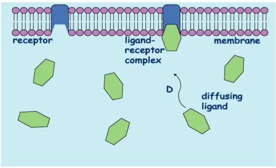
Figure 1.1 The Diffusion and Binding of Ligands at a Model Membrane ...5
Figure 1.2 Total Internal Reflection with Fluorescence Correlation Spectroscopy...9
Figure 2.1 Schematic of TIR-FCS ...18
Figure 2.2 Fluorescence Fluctuation Autocorrelation Function for Spatially Independent Diffusion ...21
Figure 2.3 Distance-Dependent Diffusion for Sphere Near a Wall ...23
Figure 2.4 Representative TIR-FCS Autocorrelation Functions ...31
Figure 2.5 Seand rSeas a Function of r...36
Figure 3.1 Stacked Bilayer System...45
Figure 3.2 FPPR Experiment ...48
Figure 3.3 Schematic of AFM ...53
Figure 3.4 Representative FPPR Recovery Curves ...65
Figure 3.5 Representative Order Parameter Curves ...68
Figure 3.6 Representative AFM Images ...71
Figure 4.1 Schematic for TIR with High Refractive Index Substrates ...79
Figure 4.2 Theoretical Plots of Eq. 2.9 ...81
Figure 4.3 Epi-fluorescence Images of Bilayers atop SiO2, TiO2, and SrTiO3...86
Figure 4.4 Total Internal Reflection on SrTiO3...87
Figure 4.5 Fluorescence Scans of SrTiO3and TiO2...89
Figure 4.6 Fluorescence Intensity vs. Concentration Plots...91
Figure 4.7 Representative Autocorrelation Function for Fluorescently Labeled IgG Antibodies atop a TiO2Prism...93
LIST OF ABBREVIATIONS 31-11 Type of IgG Antibody
1B711 Type of IgG Antibody
AbC Antibody Complex
AFM Atomic Force Microscopy
Biotin-cap-DPPE 1,2-Dipalmitoyl-sn-Glycero-3-Phosphoethanolamine-N-(Cap Biotinyl) (Sodium Salt)
Biotin-LC-DPPE N-[6-[[Biotinoyl]Amino]Hexanoyl]-Dipalmitoyl-L-N -Phosphatidylethanolamine, Triethylammonium Salt BS3 Bis(sulfosuccinimidyl) suberate
dH20 Deionized Water
DLS Dynamic Light Scattering
DMSO Dimethyl Sulfoxide
DNP Dinitrophenyl
erfc Complementary Error Function
Fab, (Fab’)2 Fragments of Antibodies that Bind Antigens and Determine their Specificity
FCS Fluorescence Correlation Spectroscopy FcORII Mouse Fc Receptor FcORII
FITC Fluorescein Isothiocyanate
LB Langmuir-Blodgett Bilayer Preparation LS Langmuir-Schafer Bilayer Preparation Mar18.5 Type of IgG Antibody
MW Molecular Weight
N.A. Numerical Aperture
NBD-PC 1-Acyl-2-[12-(7-Nitro-2-1,3-Benzoxadiazol-4-yl) Aminododecanoyl]- Glycero-3-Phophocholine
PBS Phosphate Buffered Saline
PMT Photomultiplier Tube
POPC 1-Palmitoyl-2-Oleoyl-Glycero-3-Phosphocholine SDS-PAGE Sodium Dodecylsulfate-Polyacrylamide Gel Electrophoresis STM Scanning Tunneling Microscopy
SUV Small Unilamellar Vesicles TIR Total Internal Reflection
LIST OF SYMBOLS < > time or ensemble average
a stripe periodicity in the sample plane A solution concentration of a ligand
incidence angle of the laser beam (measured normal from substrate) also the intercept (chapter 2)
c critical angle for TIR
B a measured constant in order parameter measurements B average measured blank signal for TIR-FCS
& the bleach fraction in FPPR
& also the slope (chapter 2)
'2 the chi-squared statistical goodness of a fit d depth of the evanescent wave for TIR
D diffusion coefficient
Di diffusion coefficient of the ith species in FPPR fluctuation in a quantity for TIR-FCS
F(t) fluorescence fluctuation at time tin TIR-FCS *(z-z’) a Dirac delta function
¶ extinction coefficient or molar absorptivity solvent viscosity
Fn the F-statistic associated with the nspecies model
F(t) instantaneous fluorescence intensity at time tin TIR-FCS and FPPR F( ) the pre-bleach fluorescence in FPPR
F(.) the fluorescence as a function of beam polarization angle in order parameter measurements
<F> temporally averaged fluorescence intensity for TIR-FCS G baseline correction term for data fitting in TIR-FCS G( ) fluorescence fluctuation autocorrelation function
Ge( ) autocorrelation function for diffusion through the evanescent wave Gs( ) autocorrelation function for diffusion through solution for FCS
abbreviations for parameters in Stokes-Einstein Equation (Chapter 2) 1 the dichroic factor in order parameter measurements
2 the angle that the beam polarization makes with the incidence plane in order parameter measurements
h observation area radius defined by aperture for TIR-FCS Io maximum intensity of the evanescent field
I(z) evanescent intensity
k the spring constant in AFM
ki characteristic rate for the recovery of the ith species for FPPR
k Boltzmann Constant
vacuum wavelength of laser light
mi percent mobility associated with the ith species in FPPR mo the mass that loads the spring in AFM
N the number of data points for F-statistics
n1,n2 refractive index of substrate and water, respectively
Ne average number of fluorescent molecules in the observation volume Ns average number of fluorescent molecules in the focused spot for FCS N(5) the orientation distribution of fluorophore absorption dipoles in
order parameter measurements
r hydrodynamic radius
Pi Legendre Polynomial
pi the probability value with regards to the statistical goodness of a fit R the correlation coefficient with regards to the goodness of a fit Re rate of diffusion through the evanescent wave for TIR-FCS Rs rate of diffusion through solution for FCS
s the 1/e2-radius of the focused spot for FCS
si the order parameter
Se initial slope of the autocorrelation function for diffusion through the depth of the evanescent intensity
Ss initial slope of the autocorrelation function for diffusion through a focused spot for FCS
S average measured total fluorescence signal for TIR-FCS structure parameter in FCS
t time
T absolute temperature
Chapter 1 Introduction
Throughout the centuries, science has proven itself a vast playground for the curious and imaginative. As man and womankind’s understanding of the universe has grown through their investigations, most of the simple scientific principles have been deduced. The
deduction of “simple” science has fueled a hunger for the more complex. As graduate students in science, we find ourselves embracing this complexity. Interfaces are at no loss for complexity. When two separate species or phases are forced into contact with each other,
many interesting phenomena occur. This is where proven principles break down and boundary values reap their reason. Couple the inherent complexity of an interface to the
doubly complex nature of biological material and you have a membrane.
The biological membrane mediates a myriad of functions, and it is the site of much of the interesting chemistry with regards to cellular function. Although many of the mysteries
of the biological membrane remain to be discovered, it is known to play a central role in neurotransmission (Kim and Huganir, 1999), immunological response (Ravetch and Bolland,
2001), and nutrient uptake (Zorzano et al., 2000). The membrane is central in many of these processes because it serves as a final gateway restricting what may enter and mingle with the fragile components inside the cell. It is this role as the gateway which also necessitates that
the membrane be intrinsically linked to ligand-receptor interactions. Consequently, biological membranes are complex phospholipid bilayers containing integral transmembrane
the membrane impedes the elucidation of its properties. Resultantly, simplified model membrane systems have been employed in its study.
Several different techniques have been developed to make planar supported model phospholipid bilayers. The earliest attempts date back to the early 1900’s when in 1918 Langmuir transferred a floating monolayer to a substrate (Stryer, 1995). This subsequently
led to the development of the Langmuir-Blodgett (LB) and the Langmuir-Schaefer (LS) techniques in which a bilayer is created by the successive transfer of a monolayer to a
substrate from the air/water interface (Wright et al., 1988; Tamm and McConnell, 1985). In the 1980’s the McConnell lab developed a simpler technique to produce phospholipid bilayers known as vesicle fusion (Brian and McConnell, 1984). In vesicle fusion, small
unilamellar vesicles (SUVs) are produced by tip sonication. They are then allowed to adsorb and fuse to form a bilayer. Recent advancements have produced hybrids of the two
techniques (Kalb et al., 1992). The utility of phospholipid bilayers has seen extension beyond its use as a model membrane system. Phospholipid bilayers now find application in biosensors (Pompeo, et al., 2005; Amenitsch et al, 2004), the biofunctionalization of
inorganic solids (Sackmann, 1996), and immobilization of proteins and DNA (Pompeo et al., 2005; Sackmann, 1996; Amenitsch et al., 2004).
The continued use of phospholipid bilayers in experimental settings requires that the methodology continue to grow alongside the current needs in experiments. This requires the amendment of model membrane technology to increasingly complex and stringent
surface (Spinke et al., 1992). Protecting the model membrane from the surface roughness creates more “fluid” membranes. Also, model membranes are currently limited in their
ability to mimic the biological membrane because they do not allow transmembrane proteins to retain their lateral mobility (Wagner and Tamm, 2000; Sackmann, 1996; Naumann et al.,
2002; Kühner et al., 1994; Wong, et al., 1999; Huang, 1985; Spinke et al., 1992). A
cushioning system would limit interactions between the transmembrane protein and the substrate. This could possibly allow a transmembrane protein to have lateral mobility similar
to that seen in biological membranes. Currently, several cushioning systems have been proposed (Wanger and Tamm, 2000; Sackmann, 1996; Naumann et al., 2002; Kühner et al.,
1994; Wong, et al., 1999; Huang, 1985; Spinke et al., 1992). Many involve the use of polymers and ultra-thin polymer films (Sackmann, 1996).
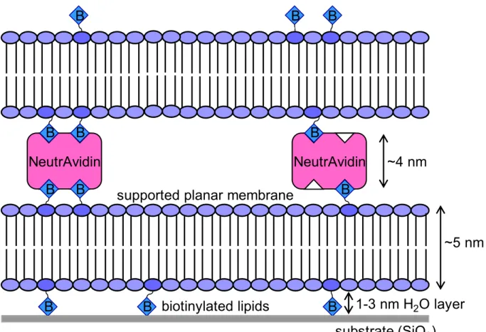
A novel approach to the development of a cushioning system is to utilize the
interactions of biotin and avidin to produce a stacked bilayer system. The utility of such a system would also see usage in multilayer applications. This stacked bilayer system has been
constructed (see Chapter 3) by first depositing phospholipid vesicles containing a small fraction of biotin onto a fused silica substrate. The biotinylated vesicles are allowed to fuse at and adsorb to the substrate. Then NeutrAvidin (a commercially available derivative of
avidin) is applied to the bilayer. Finally, biotinylated vesicles are applied atop this system and allowed to adsorb and become a bilayer. The primary bilayer and NeutrAvidin serve as
Another area requiring advancement in membrane science is the theory surrounding ligand-receptor interactions near model or cellular membranes. As was aforementioned, the
inherent gate-like nature of the biological membrane mandates that numerous different ligands diffuse up to and possibly bind to the membrane (Figure 1.1). The theory surrounding ligand-receptor interactions and their association/dissociation kinetics at
membranes has never adequately modeled what is seen experimentally (Hsieh and Thompson, 1995; Payne et al., 1997; McKiernan et al., 1987; Anderson and McConnell,
1999; Sahu et al., 2000; Domagala et al., 2000). The deviations from expectation caused scientists to postulate that other factors influence ligand translational mobility in very close proximity to membranes (see Chapter 2). One such possibility is related to physical
chemistry and the effect that the wall-like boundary of the membrane has upon the translational mobility of the ligand. If the close proximity of the membrane causes an
increase in the frictional coefficient of the ligand, the diffusion coefficient will decrease from what was previously anticipated (Forster and Lauffenburger, 1994). One way to measure the effects that the close proximity of the membrane has upon the diffusion of the ligand would
be to study ligand translational mobility as a function of ligand radii. If the membrane is effecting the diffusion of these ligands, the trend would manifest itself more for larger
Figure 1.1 The Diffusing and Binding of Ligands at a Model Membrane.
The nature of the biological membrane requires that numerous different ligands diffuse up and bind to receptors embedded in the membrane. The membrane contains many different receptor types. This schematic represents a simplified version of what is occurring.
The study of diffusion and binding near model membranes requires specialization of existing techniques so that information gathered is specific to the interface and does not
include information about bulk solution. One popular way in which this is done is by total internal reflection (TIR). Total internal reflection occurs when a plane wave traveling in a medium of higher refractive index (n1) impinges on a planar medium of lower refractive
index (n2) at an angle (defined from the normal to the interface) greater than the critical angle
(ac)
) ( sin
1 2 1
n n
C
−
=
α (1.1).
During internal reflection, the plane wave completely reflects into the higher refractive index
medium and a surface-associated evanescent wave is generated in the lower refractive index
medium (Thompson and Pero, in press). The evanescent field propagates parallel to the
of the incident light wavelength. Resultantly, a small distance from the interface (63-104 nm
at the fused silica/water interface) is selectively excited, and interactions in close vicinity to
the model membrane can be probed. The depth of the evanescent wave is defined by
2 2 2 2 1 sin
4 n n
d
− =
α π
λ
(1.2)
where d is the evanescent wave depth, l is the vacuum wavelength of light, and a is the
incident angle of the light.
Total internal reflection has been combined with many fluorescence techniques to
render them surface sensitive (Thompson and Pero, 2005). One such technique is
fluorescence correlation spectroscopy (FCS). FCS first made its debut in 1974 when other
correlation based techniques such as light scattering were being introduced (Elson and
Magde, 1974; Elson, 1985). In FCS, a small observation volume is defined by placing an
aperture (usually 50-200 mm in radius) at the confocal image plane of a microscope. By
using this small observation volume to monitor a dilute fluorescently-labeled solution
(~15-100 nM), temporal fluctuations in the measured fluorescence can yield information about the
processes giving rise to these fluctuations (Thompson, 1991). These fluctuations can be
caused by molecules moving into and out of the observation volume or changes in the
fluorescent state of molecules (singlet to triplet and vice-versa) (Elson and Magde, 1974,
Thompson, 1991; Gösch and Rigler, 2005; Fradin et al., 2005). Consequently, FCS takes
advantage of what effectively can be considered the inherent noise in a fluorescent
measurement to derive information about the molecular motion and fluorescent properties of
where F(t) is the instantaneous fluorescence intensity at time t, <F> is the average
fluorescence intensity over the course of the experiment, t is the correlation time, and dF(t)
(defined by dF(t) = F(t) - <F>) is the fluorescence fluctuation. G(t) decays monotonically
with t to zero at t = ¶. A number of recent reviews have been published describing FCS
(Vukojevic et al., 2005; Gosch and Rigler, 2005; Haustein and Schwille, 2004; Enderlein et
al., 2004; Pramanik, 2004; Weiss and Nilsson, 2004; Kahya et al., 2004; Levin and Carson,
2004; Muller et al., 2003; Hink et al., 2003; Thompson et al., 2002; Frieden et al., 2002;
Rigler and Elson, 2001).
In 1977 total internal reflection was combined with fluorescence correlation
spectroscopy (TIR-FCS) in an instrument known as a virometer (Hirschfeld and Block, 1977;
Hirschfeld et al., 1977). The virometer was a rudimentary, proof-of-principle instrument that
was devised to identify ethidium bromide stained viral molecules by their rate of diffusion
through the evanescent wave. In 1981, TIR-FCS was brought to fruition and the theory was
derived (Thompson et al., 1981). The derivation of the theory for TIR-FCS paved the way
for its application in biophysics. The advantages of using TIR-FCS as opposed to FCS are
most profound for studying dynamic processes at interfaces (Figure 1.2). By using a TIR
set-up, the technique becomes especially applicable to membrane science. However, there are
additional advantages that are useful in other aspects. For instance, FCS measurements
require that the area in which measurements be taken remain small. This is easily
accomplished in the xy plane by placing an aperture at a confocal image plane in the path of
light (Thompson, 1991). TIR increases the ability to limit sample observation volume by
making it possible to specify the z-distance that is probed by changing the incidence angle of
been used to study the kinetics of some systems, this type of FCS has some distinct
disadvantages in this area of investigation. Using FCS to probe the kinetics of two ligands
binding involved watching the change in the rate of translational diffusion upon binding.
This is not optimum because to see significant changes in translational mobility the size
increase upon binding must be of a significant magnitude, and this is rarely the case.
TIR-FCS circumvents this problem by immobilizing a nonfluorescent ligand to the surface. Then
a fluorescent ligand must diffuse into the evanescent wave and bind to a surface-immobilized
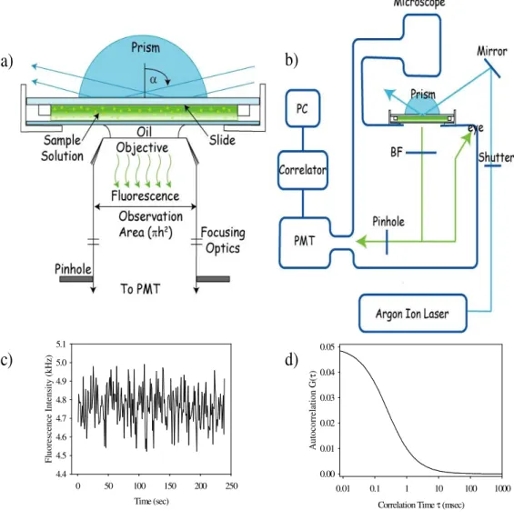
Figure 1.2 Total Internal Reflection with Fluorescence Correlation Spectroscopy.
a) Light is totally internally reflected through a fused silica prism to selectively excite molecules near the interface. b) The experimental apparatus for TIR-FCS. After light is totally internally reflected, it is sent through a pinhole at the confocal image plane. Photons are measured by a photomultiplier tube and then autocorrelated. c) The measured fluorescent intensity displays temporal fluctuations in the signal commonly referred to as noise. d) The fluorescent fluctuations are autocorrelated. The fluorescent fluctuations yield information about the movement of molecules in close proximity to the membrane and about transitions in fluorescent state.
Time (sec)
0 50 100 150 200 250
F lu o re sc e n ce I n te n si ty ( k H z) 4.4 4.5 4.6 4.7 4.8 4.9 5.0 5.1
Correlation Time τ (msec)
0.01 0.1 1 10 100 1000
A u to co rr el at io n G ( τ ) 0.00 0.01 0.02 0.03 0.04 0.05
a)
b)
c)
d)
From the advent of TIR-FCS there existed a lag time during which the technique saw
little application. However, now TIR-FCS is beginning to see abundant application and it
appears that the technique is fast becoming a staple in biophysical research. A recent review
press). However, a brief review of the use of TIR-FCS has been included here. Shortly after
the first theoretical paper, a second short theory paper was published (Thompson, 1982).
This paper hypothesized that TIR-FCS could be used to measure the surface binding kinetics
of nonfluorescent ligands competing with fluorescent ligands for the same binding sites. The
first experimental example that united the theory and TIR-FCS was when the reversible
kinetics of tetramethylrhodamine-labeled immunoglobulin and insulin interacting with fused
silica coated with serum albuminwas measured (Thompson and Axelrod, 1983).
TIR-FCS was used to measure the diffusion coefficients and concentrations of
fluorescently-labeled IgG diffusing within the depth of the evanescent wave (Starr and
Thompson, 2001; Starr and Thompson, 2002). Also, TIR-FCS was recently demonstrated to
measure the kinetics of a specific and reversible association between fluorescently labeled
ligands (IgG) in solution and their receptors (mouse FcγRII) embedded in
substrate-supported planar membranes (Lieto et al., 2003; Scwhille, 2003). This application is
noteworthy because it was the first demonstration of nonfluorescent and fluorescent ligands
(of the same type) being measured by TIR-FCS as proposed by the second theory paper
(Thompson, 1982). The next extension of this would be to monitor the binding of ligands of
different types (one fluorescently-labeled species and one unlabeled species). Although this
has not occurred to date, investigations of this nature are being proposed.
Of late, two studies monitored the diffusion of fluorescein within the evanescent
wave depth using TIR-FCS(Harlepp et al., 2004; Hassler et al., 2005). These represent the
first studies demonstrating the application of TIR-FCS by through-objective as opposed to
However, TIR-FCS has been used to monitor the motions of fluorescently labeled,
intracellular vesicles near the plasma membranes of adherent cells(Johns et al., 2001; Holt et
al., 2004).
TIR-FCS is also being extended beyond usage in the area of biophysics. TIR-FCS
has been used to monitor the reversible kinetics of rhodamine 6G interacting with
C-18-modified silica surfaces (Hansen and Harris, 1998a; Hansen and Harris, 1998b).
Subsequently, a comprehensive set of measurements employed TIR-FCS to investigate
molecular transport in substrate-supported, sol-gel films(McCain and Harris, 2002; McCain
et al., 2004a; McCain et al., 2004b).
Some recent interest in TIR-FCS has been in its use with high refractive index
substrates to generate very small evanescent waves. Smaller evanescent waves would be of
use because they would facilitate the study of systems with weaker binding constants and
provide information about chemistry occurring closer to surfaces (Thompson and Pero,
2005). Recently, it has been proven that phospholipid bilayers can be formed upon titanium
dioxide and strontium titanate (Starr and Thompson, 2000; Rossetti et al. 2005).
Consequently, the first step to amending the use of high refractive index substrates to
biophysical surface studies has been taken. Furthermore, combining high refractive index
substrates with techniques like variable angle total internal reflection (VA-TIR) will allow
depth profiling studies to be performed. VA-TIR changes the incidence angle of the
impinging laser light and produces smaller evanescent depths by Eq. 1.2.
This thesis represents the compilation of new methodologies and theories all
intrinsically related to model membranes, total internal reflection, and TIR-FCS. Their
protocols, and lead to the modification of theories governing interactions near membranes. It
is hoped that this contribution provides a stepping stone upon which future contributors may
Reproduced with permission from the American Chemical Society Copyright 2006 Pero, J.K., Haas, E.M., and Thompson, N.L. 2006 J. Phys. Chem. B. 110:10910-10918.
Chapter 2 Size Dependence of Protein Diffusion Very Close to
Membrane Surfaces: Measurement by Total Internal Reflection
with Fluorescence Correlation Spectroscopy
2.1
Abstract
The diffusion coefficients of nine fluorescently labeled antibodies, antibody
fragments and antibody complexes have been measured in solution very close to supported
planar membranes by using total internal reflection with fluorescence correlation
spectroscopy (TIR-FCS). The hydrodynamic radii (3 to 24 nm) of the nine antibody types
were determined by comparing literature values with bulk diffusion coefficients measured by
spot FCS. The diffusion coefficients very near membranes decreased significantly with
molecular size, and the size dependence was greater than that predicted to occur in bulk
solution. The observation that membrane surfaces slow the local diffusion coefficient of
proteins in a size-dependent manner suggests that the primary effect is hydrodynamic as
predicted for simple spheres diffusing close to planar walls. The TIR-FCS data are
consistent with predictions derived from hydrodynamic theory. This work illustrates one
factor that could contribute to previously observed non-ideal ligand-receptor kinetics at
model and natural cell membranes.
2.2
Introduction
The interactions of ligands with their receptors at biological interfaces such as
membranes are at the heart of many if not all biological processes including, for example,
2001), and nutrient uptake (Zorzano et al., 2000). Previous studies have indicated that the
association/dissociation kinetics of ligands in solution with receptors in natural or model
membranes are very often not adequately explained as simple, reversible, bimolecular
reactions between point particles(Hsieh and Thompson, 1995; Payne et al., 1997; McKiernan
et al., 1987; Anderson and McConnell, 1999; Sahu et al., 2000; Domagala et al., 2000).
Numerous hypotheses have been developed to account for the observed non-ideality
including models with an increased number of discrete states (Lauffenburger and
Lindermann, 1993) or models in which the system is described as containing a continuum of
bound states(Kopelman, 1988; Frauenfelder et al., 1991; Murray and Honig, 2002). Other
investigations into the molecular details of ligand-receptor kinetics have included rebinding
effects (Lagerholm and Thompson, 1998; Levin et al., 2002), rotational mobility or
orientational effects (Shoup et al., 1981; Schweitzer-Stenner et. al., 1992). An additional
possibility is that the observed non-ideality arises at least in part from deviations of the
ligand translational mobility in close proximity to membranes from the bulk diffusion
coefficient.
Total internal reflection with fluorescence correlation spectroscopy (TIR-FCS) is a
method particularly well-suited to probing molecular motions and interactions close to
surfaces. In TIR-FCS, a laser beam is internally reflected at the interface of a planar surface
and an aqueous medium. The internal reflection generates a surface-associated evanescent
field that penetrates only slightly into the aqueous medium and excites fluorescence from
molecules bound to the surface or in solution but very close to the surface. The fluorescence
out of the volume. The time-dependence of the autocorrelation function of the fluorescence
fluctuations provides information about the local translational mobility of the fluorescent
molecules and if they reversibly interact with surface sites, the kinetics associated with the
surface interaction.
The theoretical basis for using TIR-FCS to examine near-surface dynamics, including
translational diffusion in solution very close to the surface as well as the kinetics of
reversible association and dissociation with the surface, has been established(Thompson et
al., 1981; Starr and Thompson, 2001; Lieto and Thompson, 2004). A number of
experimental TIR-FCS studies have also been carried out. Initially, TIR-FCS was used to
examine the reversible kinetics of tetramethylrhodamine-labeled immunoglobulin and insulin
interacting with fused silica coated with serum albumin(Thompson and Axelrod, 1983) and
of rhodamine 6G interacting with C-18-modified silica surfaces(Hansen and Harris, 1998a;
Hansen and Harris, 1998b). Subsequently, a comprehensive set of measurements employed
TIR-FCS to investigate molecular transport in substrate-supported, sol-gel films(McCain and
Harris, 2002; McCain et al., 2004a; McCain et al., 2004b). Two recent studies monitored the
diffusion of fluorescein within the evanescent wave using TIR-FCS (Harlepp et al., 2004;
Hassler et al., 2005). The first demonstration of TIR-FCS as a method for monitoring the
kinetics of a specific and reversible association between fluorescently labeled ligands (IgG)
in solution and their receptors (mouse FcγRII) embedded in substrate-supported planar
membranes has been recently described(Lieto et al., 2003). Versions of TIR-FCS have also
been used to monitor the motions of fluorescently labeled, intracellular vesicles near the
The work described here addresses the nature of protein diffusion very near model
phospholipid membrane surfaces. The question considered is the manner in which the
membrane affects local protein diffusion and therefore might affect the kinetics of interaction
between protein ligands and their membrane-associated receptors. In a previous work,
comprehensive TIR-FCS measurements were carried out for monoclonal mouse IgG
diffusing close to substrate-supported planar model membranes(Starr and Thompson, 2002).
The main conclusion of this work was that if local electrostatic fields significantly affect
protein diffusion close to membrane surfaces, the effects are confined to distances much
smaller than 100 nm from the surface. However, this work did suggest that hydrodynamic
effects might affect protein mobility close to membrane surfaces in a manner that might be
observable even at distances extending 100 nm or more from the membrane.
Indeed, there exists a long-lived literature describing decreased diffusion of spherical
particles close to planar walls. The core of these theories is related to the development of the
notion of frictional coefficients when addressing macromolecular hydrodynamics. In these
continuum-based theoretical treatments, the frictional coefficients for sphere motion through
a viscous medium close to and both tangential or normal to the surface are increased, and the
diffusion coefficients are decreased. These effects, for spheres diffusing close to walls, have
been theoretically predicted for decades and the signature is an increased dependence of the
local diffusion coefficient on the size of the sphere(Forster and Lauffenburger, 1994). The
theoretical predictions have been experimentally verified, in part, for large colloidal particles
(Frej and Prieve, 1993; Bevan and Prieve, 2000; Lin et al., 2000; Dufresne et al., 2000;
In the work described herein, the diffusion coefficients of nine fluorescently labeled
antibody fragments, antibodies and antibody complexes (with hydrodynamic radii ranging
from 3 to 24 nm) adjacent to planar supported model membranes were measured by using
TIR-FCS. The results show that the local diffusion coefficient decreases with the
hydrodynamic radius, over and above that predicted by the Stokes-Einstein equation
describing diffusion in bulk solution, and in a manner consistent with theoretical predictions
according to hydrodynamic theories describing particle motions next to walls.
2.3
Theoretical Background
2.3.1
ApparatusA laser beam is internally reflected at a substrate/solution interface and creates an
evanescent intensity that penetrates exponentially with characteristic depth d into the solution
adjacent to the surface (Thompson and Pero, in press; Abramowitz and Stegun, 1968) (Figure
2.1). The evanescent intensity, I(z), is given by
) exp( )
( 0
d z I
z
I = − (2.1)
where z is the distance in solution from the interface, d is the depth of the evanescent wave,
and I0 is the intensity at the interface. In the measurements described here, the interface of a
fused silica substrate (refractive index n1= 1.467) and an aqueous salt solution (refractive
index n2≈ 1.337) (Starr and Thompson, 2002) is illuminated by a 488.0 nm laser line. For
these refractive indices, the critical angle for internal reflection is αC = 65.7o. Thus, the
evanescent depth ranges from d≈ 105 nm to d≈ 65 nm. Fluorescence is collected through a
60x, 1.4 N.A. objective. The evanescent intensity along with a small circular aperture (50
μm radius) placed at an intermediate image plane of a microscope, corresponding to a radius
h≈ 1 μm in the sample plane, defines a small observation volume.
Figure 2.1Schematic of TIR-FCS.
A small sample volume is defined by the depth of the evanescent intensity, d, in combination with a circular aperture placed at an intermediate image plane of the microscope that defines an area of radius h in the sample plane. The fluorescence measured from the small sample volume adjacent to the surface fluctuates with time as molecules diffuse close to the surface, and the fluorescence fluctuations are autocorrelated.
aperture
focusing optics observation
area (h2)
to detector
2.3.2 Fluorescence Fluctuation Autocorrelation Function G(τ)
Individual fluorescent molecules in solution diffuse into and out of the defined
observation volume. Their motion causes the measured fluorescence to fluctuate with time.
These fluctuations are defined as the difference between the instantaneous fluorescence
intensity, F(t), and its time-averaged value, <F>; i.e., δF(t) = F(t) - <F>. The fluorescence
fluctuations are autocorrelated to obtain information about the diffusion of fluorescent
molecules in the observation volume. The fluorescence fluctuation autocorrelation function
is defined as
2 2 ) 0 ( ) ( ) ( ) ( ) ( > < > < = > < > + < = F F F F t F t F
Gτ δ τ δ δ τ δ (2.2)
2.3.3 Magnitude of the Fluorescence Fluctuation Autocorrelation Function
As shown previously (Starr and Thompson, 2001), if the concentration of fluorescent
molecules in solution does not depend on z, as we assume here, the magnitude of the
fluorescence fluctuation autocorrelation function (Ge(0)) is
e e N G 2 1 ) 0
( = (2.3)
where Ne is the average number of fluorescent molecules in the observed volume, defined
dA h
Ne =π 2 (2.4)
Ge(0) is inversely related to the solution concentration A.
2.3.4 Shape of the Fluorescence Fluctuation Autocorrelation Function for Spatially
Independent Diffusion.
In this work, we assume that the sample volume radius along the surface, h, is much
greater than the evanescent depth, d. When the diffusion coefficient, D, does not depend on z,
the theoretical form of the TIR-FCS fluorescence fluctuation autocorrelation function is
(Starr and Thompson, 2001)
⎭ ⎬ ⎫ ⎩ ⎨ ⎧ − +
= (0) (1 2 )exp( ) [( )1/2] 2( )1/2
) ( π τ τ τ τ τ e e e e e e R R erfc R R G
G (2.5)
where πη γ γ 6 & 2 2 kT r d d D
Re = = = (2.6)
Here, Re is the rate for diffusion in solution through the depth of the evanescent intensity, r is
the hydrodynamic radius, k is Boltzmann’s constant, T is the absolute temperature, and η is
the solution viscosity. As shown in Figure 2.2a, Ge(τ)/Ge(0) decays monotonically with time.
e e e e R G G d d S = ⎭ ⎬ ⎫ ⎩ ⎨ ⎧ = =0 ] ) 0 ( ) ( [ τ τ
τ (2.7)
The time at which Ge(τ) equals one half of its initial value is 3.3 Re-1.
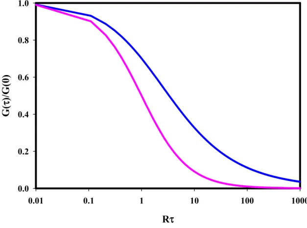
Figure 2.2 Fluorescence Fluctuation Autocorrelation Function for Spatially Independent Diffusion.
G(τ)/G(0) decays with time. The blue line shows Ge(τ)/Ge(0) for evanescent illumination
(Eq. 2.5). In this case, the initial slope is –Re and the half-time for decay is 3.3 Re-1. The
pink line shows Gs(τ)/Gs(0) for illumination with a focused spot in solution (Eq. 2.12). In
this case, the initial slope is –Rsand the half-time for decay is Rs-1.
R
τ
0.01 0.1 1 10 100 1000
G(
τ
)/G(0)
0.0 0.2 0.4 0.6 0.8 1.02.3.5 Spatially Dependent Diffusion Coefficients
In this work, we are particularly concerned with the situation in which the diffusion
coefficient depends on the distance from the interface. We test the hypothesis that the
hydrodynamic effects. In this case, even in the absence of local potentials, this coefficient is
predicted to depend on z (and the sphere radius, denoted here by r) for a sphere diffusing next
to a wall. The predicted form of D(z, r), for diffusional motion normal to the interface, is
(Brenner, 1961; Lin et al., 2000; Oetama and Walz, 2005)
⎪ ⎪ ⎭ ⎪⎪ ⎬ ⎫ ⎪ ⎪ ⎩ ⎪⎪ ⎨ ⎧ − + + − + + + + + + + + − + + = − − − − ∞ = −
∑
1 )] 1 ( [cosh sinh ) 1 2 ( )] 1 ( cosh ) 5 . 0 [( sinh 4 )] 1 ( cosh 2 sinh[ ) 1 2 ( )] 1 ( cosh ) 1 2 sinh[( 2 ) 3 2 )( 1 2 ( ) 1 ( )] 1 ( sinh[cosh 3 4 ) , ( 1 2 2 1 2 1 1 1 1 r z k r z k r z k r z k k k k k r z r z D D k (2.8)where r is the particle radius, z is the distance between the sphere edge and the wall, and
D(∞, r) = D is the diffusion coefficient in the bulk far from the wall. A much simpler,
approximate form for Eq. 2.8 has been reported(Sholl et al., 2000) as
2 2 2 2 9 6 2 6 ) , ( r rz z rz z D r z D + + +
= (2.9)
Numerical calculations show that Eqs. 2.8 and 2.9 deviate by no more than 0.6%. The
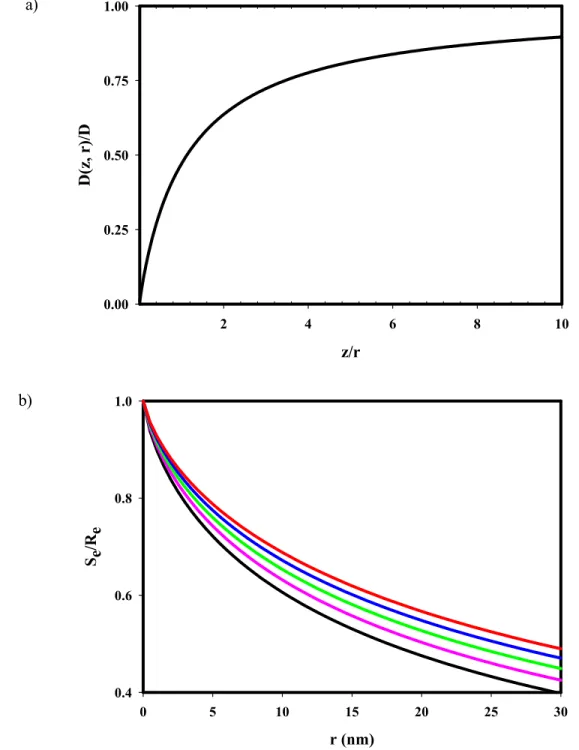
Figure 2.3 Distance-Dependent Diffusion for a Sphere Near a Wall.
(a) The diffusion coefficient as a function of the sphere radius r and the distance from the wall z increases from zero at the wall to the bulk diffusion coefficient as z approaches infinity. This plot was calculated from Eq. 2.9 and also equals Eq. 2.8. The distance for which D(z,r) = (1/2)D is z/r = (5+731/2)/12=1.13. (b) The value of Eq. 2.10 (with Eq. 2.9), calculated numerically, is shown for particle radii ranging from 0 ≤ r ≤ 30 nm and for evanescent depths of (black) d = 65 nm, (pink) d = 75 nm, (green) d = 85 nm, (blue) d = 95 nm and (red) d = 105 nm. The effect on Se/Re is more prominent for larger radii and thinner
evanescent wave depths.
a)
b)
z/r
2 4 6 8 10
D(
z,
r)
/D
0.00 0.25 0.50 0.75 1.00
r (nm)
0 5 10 15 20 25 30
Se/ Re
2.3.6 Shape of the Fluorescence Fluctuation Autocorrelation Function for Spatially
Dependent Diffusion
The generalization of Eq. 2.5 for the case in which the diffusion coefficient depends
on z is not known. However, as shown in the Appendix, if D(0) = 0 (see Eq. 2.9), the
magnitude of the initial slope of the normalized fluorescence fluctuation autocorrelation
function is ⎪ ⎪ ⎭ ⎪ ⎪ ⎬ ⎫ ⎪ ⎪ ⎩ ⎪ ⎪ ⎨ ⎧ − − =
∫
∫
∞ ∞ 0 0 ) 2 exp( ) , ( ) 2 exp( ) ( dz d z dz D r z D d z R rSe e (2.10)
where Re is given by Eq. 2.6. The value of Se/Re was calculated numerically from Eqs. 2.9
and 2.10 and is shown in Figure 2.3b. The ratio Se/Redecreases for larger particle radii and
for thinner evanescent wave depths. Remarkably, Se is predicted to be measurably less than
that for pure bulk diffusion, Re, even in cases where the particle radius is significantly less
than the evanescent wave depth.
2.3.7 Fluorescence Correlation Spectroscopy with a Focused Spot in Solution
In some measurements, the bulk diffusion coefficients of different protein
preparations were examined by carrying out fluorescence correlation spectroscopy far from
the membrane surface. In these measurements, the sample volume was defined by tightly
focusing the laser beam and aligning a confocal pinhole in a back image plane. In this case
where Ns is the average number of molecules in the new sample volume. The shape of the
fluorescence fluctuation autocorrelation function is approximated as (see Methods)
τ τ s R + ≈ 1 (0) G ) ( G s
s (2.12)
where
r s s
D
Rs = 42 = 42γ (2.13)
s is the 1/e2-radius of the focused spot and γ is defined in Eq. 2.6 (Figure 2.2b). The
magnitude of the initial slope is
s s s s R G G d d S = ⎭ ⎬ ⎫ ⎩ ⎨ ⎧ = =0 ] ) 0 ( ) ( [ τ τ
τ (2.14)
2.4 Materials and Methods
2.4.1 Antibody Preparation
Antibodies of the type IgM (Sigma-Aldrich, St. Louis, MO), IgA (Sigma-Aldrich),
IgG F(ab’)2 (Jackson ImmunoResearch Laboratories, Inc., West Grove, PA), and IgG Fab
(Jackson ImmunoResearch Laboratories) were dialyzed into phosphate-buffered saline (PBS;
0.05 M sodium phosphate, 0.15 M NaCl, pH 7.4). IgG antibodies were obtained from the
anti-dinitrophenyl mouse-mouse hybridoma 1B711 (American Type Culture Collection,
Rockville, MD), the anti-rat IgG mouse-mouse hybridoma MAR18.5 (American Type
Culture Collection), and the anti-Thy-1 rat-mouse hybridoma 31-11 (Gerald J. Spangrude,
University of Utah, Salt Lake City). Hybridomas were maintained in culture and the
secreted antibodies were purified from cell supernatants by affinity chromatography with
DNP-conjugated human serum albumin for 1B711 antibodies(Starr and Thompson, 2002),
with Protein G for MAR18.5 antibodies, and with MAR18.5 for 31-11 antibodies(Poglitsch
and Thompson, 1990). For MAR18.5 purification, the wash buffer was PBS and the elution
buffer was 0.1 M glycine, 0.01% NaN3, pH 2.7. Each liter of supernatant yielded
approximately 10-15 mg of antibody as determined spectrophotometrically by assuming that
the molar absorptivity at 280 nm was 1.4 mL mg-1 cm-1. All antibodies were subjected to SDS-PAGE with silver staining and FPLC-dynamic light scattering to ascertain their purity.
Covalently conjugated antibody complexes (AbC’s) were engineered to make
molecules of differing radii than those found naturally and provide a broader range of
molecular sizes to study. 31-11 antibodies were mixed with MAR18.5 antibodies at a 2:1
PBS. Bis(sulfosuccinimidyl) suberate (BS3) (Pierce Biotechology, Rockford, IL) was then added to the antibodies in a 20-120 molar excess to bind the antibodies together and prevent
equilibrium dissociation. The reaction with BS3 was carried out for 30 minutes and then quenched with 25-45 mM glycine, at room temperature. The mixture was then dialyzed
againstPBS at 4oC to remove excess glycine and BS3.
The mixture of antibody complexes was then subjected to SDS-PAGE analysis with
silver staining to determine the number of products formed. The gels indicated that a broad
range of products had been created. This mixture of AbC’s was dialyzed into PBS with 0.5
M NaCl and passed through a 0.2 μm filter. The AbC’s were separated using an ÄKTA
FPLC interfaced with a Tricorn Superose 6 column (Amersham Biosciences, Piscataway,
NJ). The FPLC was operated at a flow rate between 0.4-0.5 mL/min and 0.5 mL fractions
were collected. Analysis of the chromatographic trace revealed that the separation was
incomplete and produced one broad peak. Numerous separations were performed under the
same conditions and the eluents were pooled fraction by fraction. The broad peak was
divided into five groups. The first of the five groupswas discarded as it contained extremely
large AbC’s. The remaining four groups were dialyzed into PBS and named AbC1, AbC2,
AbC3, and AbC4 with AbC1 being the largest and first to elute and AbC4 being the smallest
and last to elute.
All antibodies and AbC’s were fluorescently labeled using the AlexaFluor488 Protein
Labeling Kit (Molecular Probes, Inc., Eugene OR). The free dye was removed by using size
exclusion chromatography with Sephadex G-25 or G-50 in PBS. The molar concentrations
of antibody or AbC and the molar ratios of AlexaFluor488 to antibody or AbC (0.5-9
protocol. The molar extinction coefficients (in M-1cm-1) for the antibodies and antibody complexes were approximated by multiplying 1.4 L/cm g by the estimated molecular
weights. The estimated molecular weights for the AbCs were determined by using a Wyatt
DAWN EOS light scattering instrument interfaced to an Amersham Biosciences ÄKTA. As
described above, the FPLC separation was incomplete. Consequently, the peak was split into
five segments, the first segment was excluded, and the light scattering software was used to
determine an average molecular weight for the remaining four segments. Immediately
before use, Fab, F(ab’)2, IgG, and AbC4 were clarified using 0.1 μm and then 0.02 μm
filters;IgM, IgA, AbC1, AbC2, and AbC3 were clarifiedusing 0.2 μm filters.
2.4.2 Phospholipid Vesicles
Small unilamellar vesicles of 1-palmitoyl-2-oleoyl-glycero-3-phosphocholine (POPC)
(Avanti Polar Lipids, Birmingham, AL) were prepared by tip sonication of 2 mM
suspensions of POPC in water as previously described (Lagerholm et al., 2000). In some
experiments, 2 mol% of the fluorescent lipid 1-acyl-2-[12-(7-nitro-2-1,3-benzoxadiazol-4-yl)
aminododecanoyl]-glycero-3-phophocholine (NBD-PC) was included to monitor bilayer
formation and quality (see below). Vesicle suspensions were clarified by air
ultracentrifugation (130000g, 30 min) immediately before use.
2.4.3 Substrate-Supported Phospholipid Bilayers
Substrate-supported planar phospholipid bilayers were formed as previously
described(Starr and Thompson, 1993). Fused silica substrates were cleaned extensively by
boiling in detergent (ICN, Aurora, OH), bath sonicating, rinsing thoroughly with deionized
by applying 75 μL of the vesicle suspension to a fused silica substrate (1 h, 25 °C), and
rinsing with 3 mL of PBS. Fluorescence imaging microscopy and fluorescence pattern
photobleaching recovery indicated that bilayers containing NBD-PC were continuous and
fluid. For TIR-FCS measurements, bilayers without NBC-PC were treated with 400 μL of
15-90 nM antibody or AbC in PBS. For FCS experiments with a focused spot, bilayers
without NBC-PC were treated with a mixture of 3 nM antibody or AbC and 27 nM
unlabelled antibody or AbC.
2.4.4 Fluorescence Microscopy
TIR-FCS and FCS with a focused spot were carried out on an instrument consisting
of an argon ion laser (Innova 90-3; Coherent, Palo Alto, CA), an inverted microscope (Zeiss
Axiovert 35), and a single-photon counting photomultiplier (RCA C31034A, Lancaster, PA).
All experiments were conducted at 25 °C using the 488 nm laser line. For TIR-FCS
measurements, the laser beam was s-polarized while incident on the fused silica/aqueous
interface and generated an evanescent field polarized parallel to the interface. The incidence
angle was ≈ 71-85°, corresponding to theoretically predicted evanescent wave depths ranging
from 105-65 nm (see above). For conventional FCS measurements, the laser beam was
focused in the protein solution approximately 20 μm from the bilayer surface to form a small
Gaussian-shaped illumination with a radius on the order of s≈ 1 μm.
In both TIR-FCS and focused beam experiments, a pinhole with a radius of 50 μm
placed at an internal image plane defined an area with a radius of h ≈ 1μm when projected
onto the sample plane. The fluorescence arising from the volume defined by the excitation
light and the pinhole was collected through a 60x, 1.4 N.A. objective. The fluorescence
Autocorrelation functions were obtained within 5-10 min using incident laser intensities of
4-17 μW/μm2 for TIR-FCS experiments or 5-30 μW/μm2 for FCS experiments using the focused beam. The resulting evanescent intensities at the interface differed by a factor of ≈
0.2-2.5. (Thompson et al., 2005) Average blank signals were measured from samples containing buffer adjacent to supported bilayers. Possible detector afterpulsing was
examined by using a published procedure(Hillesheim and Muller, 2005). The measurements
demonstrated that any afterpulsing present was extremely minimal and in any case much
faster that the time range of the TIR-FCS data (see Figure 2.4).
2.4.5 Data Analysis
Autocorrelation functions were background-corrected by multiplying by the factor
〈S〉2/〈F〉2, where 〈F〉 = 〈S〉 - 〈B〉 was the average fluorescence calculated by subtracting the
average measured blank signal 〈B〉 from the average measured total signal 〈S〉(Thompson,
1991). TIR-FCS autocorrelation functions were fit to Eq. 2.5 with Eq. 2.3 plus an arbitrary
constant G∞, and the free parameters were Re, Ne, and G∞. Autocorrelation functions
measured using the focused beam were fit to Eq. 2.12 with Eq. 2.11 plus an arbitrary constant
G∞, and the free parameters were Rs, Ns, and G∞. For spot FCS measurements, the more
general expression, Gs(τ)≈Gs(0)[1+Rsτ]-1[1+(Rsτ/σ2)]-1/2, where σ is the “structure
parameter”, may also be used for data analysis. However, the value of σ in our apparatus is
approximately three, and the second factor in the more general expression is negligible(Allen
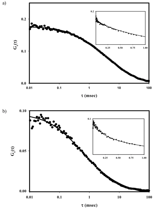
Figure 2.4 Representative TIR-FCS Autocorrelation Functions.
The background-corrected Ge(τ) are for (a) AbC1 or (b) AbC4 in PBS adjacent to a POPC
membrane. The fluorescence was monitored and autocorrelated for 300 s. The average signals 〈S〉 and background intensities 〈B〉 were (a) 10.61 & 0.04 kHz and (b) 10.03 & 0.19 kHz. The best fits of these particular functions to Eq. 2.5 with Eq. 2.3 gave (a) Ne = 2.55, Re
= 0.826 ms-1; and (b) Ne = 4.81, Re = 4.51 ms-1. Note that the theoretical curves accurately
find the initial slope (insets).
τ (msec)
0.01 0.1 1 10 100
G e
(
τ
)
0.0 0.1 0.2
0.25 0.50 0.75 1.00
0.2
a)
b)
τ (msec)
0.01 0.1 1 10 100
Ge
(
τ
)
0.00 0.05 0.10
0.25 0.50 0.75 1.00
2.5 Results
As viewed through a 1.4 N.A. objective using evanescent illumination, samples
consisting of soluble antibodies or AbC’s near planar model POPC membranes displayed
visually apparent fluorescence fluctuations which appeared as fluorescent twinkles against a
uniform background. The temporal fluctuations in fluorescence, as measured through a small
pinhole at a back image plane (Figure 2.1), were autocorrelated (Eq. 2.2). These TIR-FCS
measurements were carried out for nine antibodies or AbC’s. Correlation functions for
matched samples not containing fluorescent solutes were not measurable.
Background-corrected TIR-FCS autocorrelation functions, Ge(τ), were fit to Eq. 2.5
(with Eq. 2.3) plus an arbitrary constant G∞, with free parameters Ne, Re, and G∞. Typical
experimentally obtained Ge(τ) and their best fits to this theoretical form, for two of the nine
samples, are shown in Figure 2.4. The best-fit values of the arbitrary offset, G∞, were on the
average less than ∼10% in magnitude compared to the best-fit values of Ge(0). The best-fit
values of Ne ranged from ∼2 to 20, consistent with the expected values of Ne for solution
concentrations A = 15-90 nM, an evanescent wave depth d = 85 nm (see below) and an
observation area radius h = 1.0 μm (Eq. 2.4). The best fit-values of Re ranged from 7.8 ms-1
to 0.8 ms-1 and decreased systematically with molecular size, consistent with expectations. To ensure that the TIR-FCS data did not show photoartifacts, the incident intensity was kept
between 4 and 17 μW/μm2 (Starr and Thompson, 2002) and G
e(τ) were measured for at least
two different incident intensities. No significant change in the best-fit parameters was
The form of this function is unknown, but the magnitude of its initial slope Se is predicted by
Eq. 2.10 (see Appendix). Thus, it is important to note that the best-fits of the experimental
autocorrelation functions to Eq. 2.5 accurately find the initial slope (Figure 2.4), upon which
further analysis is based. Both the magnitude of the initial slope Se and the characteristic
time for decay of Eq. 2.5 are equal to Re (Eqs. 2.6 and 2.7).
Conventional FCS measurements with a focused spot were carried out in solutions
adjacent but not close to planar membranes, on each of the nine sample types, to determine
the hydrodynamic radii of the AbC molecules and the IgA molecule. These autocorrelation
functions were background-corrected and the resulting functions Gs(τ) were fit to Eq. 2.12
(with Eq. 2.11) plus an arbitrary constant G∞, with free parameters Ns, Rs and G∞.
Hydrodynamic radii for IgG Fab, IgG (Fab’)2, IgG and IgM were taken from the literature
(Armstrong et al., 2004). The literature value for the IgA radius was not included because it
was for monomeric IgA and dynamic light scattering measurements (see Methods)indicated
that the IgA used here was dimeric and trimeric in form. At room temperature in aqueous
solution, γ ≈ 218 μm2-nm-s-1 (Eq. 2.6). Linear regression of the measured values of Rs as a
function of the inverse of the four literature values of r (Eq. 2.13) implied 4γs-2 = 793.9 nm s
-1, consistent with a (reasonable) s value of ≈1 μm. The constant 4γs-2 was then used with the
other measured values of Rs and Eq. 2.13 to determine the radii of the AbC’s and IgA (Table
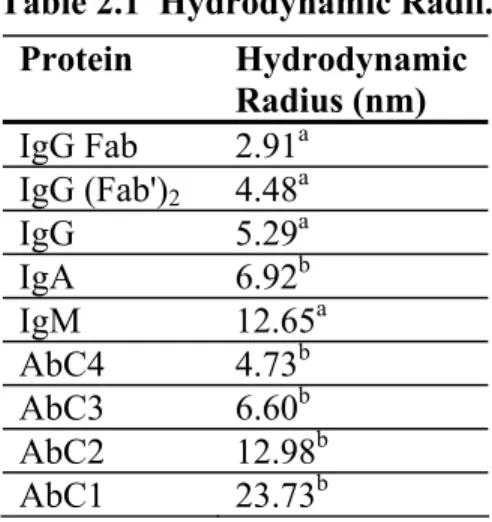
Table 2.1 Hydrodynamic Radii.
Diffusion rates in bulk solution, Rs, were determined for all nine molecule types by using
conventional FCS with a spot focused far from the membrane surface. aIgG Fab, IgG (Fab’)2, IgG, and IgM radii are from the literature (Armstrong et al., 2004). The average
measured values of Rs for these four molecules were plotted against the reciprocal of their
radii and used to find a best- fit value for the constant 4γs-2 (Eqs. 2.6 and 2.13). bThe best-fit
value of this constant was used with Eq. 2.13 to determine the radii r for the remaining five molecules, IgA and AbC1-4.
For the three molecules with the smallest literature-derived molecular radii (Fab,
(Fab’)2 and IgG) there should be only small surface effects and their bulk diffusion
coefficients can be estimated by using the measured values of Re and D = Red2 (Eq. 2.6). For
evanescent wave depths ranging from 80 to 90 nm, these calculations implied D values of
50-63 μm2s-1, 36-45 μm2s-1, and 29-37 μm2s-1, respectively. These values are in good agreement with expectations (i.e., slightly lower than) the values predicted by D = γr-1 (Eq. 2.6) and the hydrodynamic radii given in Table 1, which are 75 μm2s-1, 49 μm2s-1, and 41 μm2s-1.
The average best-fit values of Re( = Se) for each of the nine sample types are shown as
a function of the hydrodynamic radius in Figure 2.5a. As expected, Se decreased
significantly with increasing molecular size. In addition, the Se values agreed very well with
the values predicted by Eqs. 2.6, 2.9 and 2.10. These predicted values are also shown in
Protein Hydrodynamic Radius (nm)
IgG Fab 2.91a
IgG (Fab')2 4.48a