The Effects of Controlling for Distributional Differences on the Mantel-Haenszel Procedure
Daniel F. Bowen
A thesis submitted to the faculty of the University of North Carolina at Chapel Hill in partial fulfillment of the requirements for the degree of Master of Arts in the School of Education.
Chapel Hill 2011
Approved By: Dr. Gregory Cizek
ABSTRACT
Daniel F. Bowen: The Effects of Controlling for Distributional Differences on the Mantel-Haenszel Procedure
(Under the direction of Dr. Gregory J. Cizek)
Propensity score matching was used to control for the distributional differences in ability between two simulated data sets. One data set represented English speaking
ACKNOWLEDGEMENTS
I would like to thank all my colleagues in the psychometric department at Measurement Inc., especially Dr. Kevin Joldersma for working with me as we attempted to understand
TABLE OF CONTENTS
LIST OF TABLES ... vii
LIST OF FIGURES ... ix
Chapter Introduction ...1
Literature Review...9
Item Response Theory ...10
Logistic Regression ...13
The Mantel-Haenszel Chi-Square Procedure ...14
The use of Mantel-Haenszel for indentifying DIF. ...15
Mantel-Haenszel test-statistic. ...16
Mantel-Haenszel odds ratio. ...17
ETS DIF classification rules. ...17
Benefits of using Mantel-Haenszel in DIF detection. ...18
Research on the Mantel-Haenszel Procedure and Sample Size. ...19
Research on the Mantel-Haenszel Procedure and Ability Distribution Differences. ...20
Using DIF for Translated Tests ...21
Propensity Score Matching ...22
Greedy Matching. ...23
Optimal Matching. ...23
Summary ...25
Research Question ...27
Method ...28
Variables in Study ...28
Sample Size. ...28
Ability Distributions. ...28
Amount of DIF. ...29
Data Analyses ...30
Propensity Score Matching. ...31
Summary ...33
Results ...35
Simulated Data ...35
Type I Errors ...39
Type II Errors ...40
Effects on Type I Errors ...42
Effects on Type II Errors ...43
ETS Classification Agreement Rates ...44
Discussion ...47
Implications of Findings ...47
Type I Errors. ...47
Type II Errors. ...48
Effects on Type I Errors ...49
ETS Classification Agreement Rates ...52
Summary of Implications of Findings ...56
Limitations ...56
Suggestions for Future Research ...58
Conclusions ...61
Appendix A: Simulated Item Parameters and DIF Levels...62
Appendix B: SAS Code ...63
Appendix C: Item Analysis ...80
LIST OF TABLES
Table 1: Simpson’s Paradox Example ...9
Table 2: Contingency table at score point J ...16
Table 3: Total Test Score Descriptive Statistics for Simulated Data Sets ...30
Table 4: Total Test Score Descriptive Statistics for Simulated Data Sets After Matching ....32
Table 5: Descriptive Statistics of Item Difficulties of Simulated Data Sets ...36
Table 6: Descriptive Statistics of Item Difficulties of Simulated Data Sets Post-Matching ..37
Table 7: Descriptive Statistics of Point-Biserial Correlation: Pre and Post-Matching ...38
Table 8: Summary of Cronbach’s Alpha Reliability Estimates and SEMs for each Simulated Data Set ...38
Table 9: Contingency Table for Type I Errors...39
Table 10: Total Number of Type I Errors ...40
Table 11: Contingency Table for Type II Errors ...41
Table 12: Total Number of Type II Errors ...41
Table 13: Analysis of Variance for Type I Errors ...43
Table 14: Analysis of Variance for Type II Errors ...43
Table 15: Distribution of A, B, & C Class items for both Pre- and Post-Matching ...44
Table 16: ETS Classification Contingency Table – Sample Size = 1000; DIF Level = Low ...45
Table 17: ETS Classification Contingency Table – Sample Size = 500; DIF Level = Low ...45
Table 19: ETS Classification Contingency Table – Sample Size = 1000;
DIF Level = High ...46
Table 20: ETS Classification Contingency Table – Sample Size = 500; DIF Level = High ...46
Table 21: ETS Classification Contingency Table – Sample Size = 250; DIF Level = High ...46
Table 22: Total Number of Type I Errors in ETS Classification ...53
Table 23: Total Number of Type II Errors in ETS Classification ...55
Table A1: Simulated Item Parameters and DIF Levels ...62
Table C1: Item Analysis: Focal Group = 1000; DIF=Low ...80
Table C2: Item Analysis: Focal Group = 500; DIF=Low ...82
Table C3: Item Analysis: Focal Group = 250; DIF=Low ...84
Table C4: Item Analysis: Focal Group = 1000; DIF=High ...86
Table C5: Item Analysis: Focal Group = 500; DIF=High ...88
LIST OF FIGURES
Figure 1: ICCs with Similar Item Parameters ...11
Figure 2: ICCs with Differing Item Parameters ...12
Figure 3: ICCs Displaying Non-Uniform DIF ...13
Figure 4: Interaction of DIF Level and Method in Type I Errors ...51
Introduction
Tests are a vital part of a functioning society (Mehrens & Cizek, 2001). For example, when getting a physical examination, tests of blood pressure, eyesight, or hearing might be administered. The results of those tests allow the doctor to evaluate the patient and decide whether he or she needs blood pressure medication, glasses, or a hearing aid. However, imagine the results of those tests were only valid for certain segments of the population, such as an eyesight examination that yielded accurate information only for people with blue eyes. Such a result would mean that people with brown eyes would potentially be misdiagnosed or treated inappropriately. Thus, it is important that medical tests--indeed, all tests--are
routinely evaluated so that they are accurate for all segments of the population.
Analogously, in the development of any psychological or educational test, an
APA, NCME, 1999; hereafter Standards), validity is ―the most fundamental consideration in developing and evaluating tests‖ (p. 9).
One potential threat to the validity of scores is bias. The Standards (AERA, APA, NCME, 1999) states that test bias occurs “when deficiencies in a test itself or the manner in
which it is used result in different meanings for scores earned by members of different
identifiable subgroups” (p. 74). One frequent underlying cause of test bias is the
differentiation of examinees based on a characteristic that is irrelevant to the construct being
measured (i.e. construct-irrelevant variance). Construct-irrelevant variance arises from systematic measurement error. It consistently affects an examinee’s test score due to a
specific trait of the examinee that is irrelevant to the construct of interest (Hadalyna &
Downing, 2004). Dorans and Kulick (1983) used the following example to show
construct-irrelevant variance in an analogical reasoning item that appeared on the SAT:
Decoy: Duck:
(A) net:butterfly (B) web:spider (C) lure:fish (D) lasso:rope (E) detour:shortcut
Dorans and Kulick found the item to be more challenging for females than males of equal
ability. They attributed this discrepancy to male knowledge of hunting and fishing activities,
knowledge that is irrelevant to the analogical reasoning construct being measured. No test
can ever be completelyfree of bias (Camilli & Shepard, 1994). Crocker and Algina (1986)
posited that test scores will always be subject to sources of construct-irrelevant variance.
However, when the construct-irrelevant variance differs substantially between two subgroups
contributes to the reduced validity of the inferences made from test scores. By performing
statistical analyses (i.e., DIF analyses) on the items of a test, problematic items measuring
differently for different groups of examinees may be identified and test bias can be
addressed.
Presently, test developers are translating examinations into multiple languages to accommodate diverse populations of examinees, and the need for test translations is increasing, especially in elementary and secondary education contexts. For instance, the Israeli Psychometric Entrance Test (PET) was developed in Hebrew and then subsequently translated into five languages: Russian, Arabic, French, Spanish, and English. However, simply translating a test from one language to another does not automatically result in equivalent test forms (Angoff & Cook, 1988; Robin, Sireci, & Hambleton, 2003; Sireci, 1997). The test translation process may produce items that function differently across language groups. For instance, Allalouf, Hambleton, and Sireci (1999) noted that examinees who received the Russian version of the PET tended to perform at a higher level on analogy items than examinees of equal ability taking the Hebrew version. To explain the differences between the items, the test translators noted that the Russian language contains fewer
bias are recommended. One of the standard approaches for identifying item bias is DIF analysis (Zumbo, 1999).
It is important to distinguish between DIF and item bias. Zumbo (1999) defined the
occurrence of item bias as "when examinees of one group are less likely to answer an item
correctly (or endorse an item) than examinees of another group because of some
characteristic of the test item or testing situation that is not relevant to the test purpose" (p.
12). However, DIF is defined as "when examinees from different groups show differing
probabilities of success on (or endorsing) the item after matching on the underlying ability
that the item is intended to measure" (p. 12). Thus, not all items that show DIF are biased,
but all items that are biased show DIF.
To illustrate, imagine two classrooms of examinees of equal ability who receive the
same test. Class 1 has the answer to question 5 accidentally posted in classroom decorations.
Class 2 does not receive that advantage. Examinees in Class 1 are likely to perform better on
question 5 than their colleagues in Class 2, irrespective of the examinees latent ability on the
construct. DIF analysis is the process of statistically determining the differing probabilities
for success – after controlling for ability – of the two classes of examinees on question 5.
The systematic measurement error favoring examinees in Class 1 over Class 2 on question 5
is item bias. An item displaying DIF does not necessarily mean that it is inherently biased in
favor of one group or another. Often, DIF will not have a satisfactory explanation as could
be found in the example above. Ideally, DIF analysis will be used to identify items that are
functioning differently for different groups (Camilli, 2006).
against a subgroup of test takers (Camilli, 2006; Zumbo, 1999). Some degree of DIF is
almost always present. However, once DIF reaches a certain point, it threatens the validity of
test score interpretations (Robin et al., 2003). There are many statistical methods for
identifying DIF available to researchers, including methods based in classical test theory
(CTT), item response theory (IRT), and observed-score methods such as logistic regression,
Mantel-Haenszel, SIBTEST, and the standardized approach (Camilli, 2006; Camilli &
Shepard, 1994; Crocker & Algina, 1986); however, as will be discussed, most are inadequate
for validating the inferences based on test translations and adaptations.
Test translations and test adaptations are terms that are routinely used
interchangeably. Hambleton (2005) has emphasized the differences between the two.
Translating a test from one language to another is only one step in the process of test
adaptation. To adapt the test to another language translators must identify “concepts, words
and expressions that are culturally, psychologically, and linguistically equivalent in a second
language and culture.” (p. 4). Inconspicuous changes in the difficulty of vocabulary words or
the complexity of sentences can have a profound impact on the difficulty of items and
negatively affect the comparability of test adaptations. For instance, Hambleton (1994)
provided this example of an item translated from English into Swedish:
Where is a bird with webbed feet most likely to live?
In the Swedish translation the phrase “webbed feet” was translated as “swimming feet,”
providing Swedish examinees an obvious cue to the correct answer (C). Not surprisingly, the
test translation process changed the difficulty of the item.
As mentioned previously, there is an increasing need for tests to be translated from one language to another. There are large-scale test adaptation projects underway in the United States with the National Assessment of Educational Progress (NAEP) (Hambleton, 2005) and the SAT (Muniz et al., 2001). In the European Union there are 20 official languages and 30 minority languages that are acknowledged by the European Charter of Fundamental Rights (Elousa & Lopez-Jaregui, 2007) and efforts are underway to translate educational assessments to accommodate that diverse population.
Validating inferences made from the administration of translated tests poses unique problems for educational researchers. In many cases the population that has received the accommodation to adapt the test to their native language (i.e., the focal group) will be much smaller than the population taking the test in its original language (i.e., the reference group) (Robin et al., 2003). Traditional methods for detecting DIF are not suitable for detecting DIF accurately when there are large discrepancies between reference and focal groups in sample size, ability level, or dispersion (Hambleton et al., 1993) or when the combined sample size is small (Muniz et al., 2001). Mazor, Clauser, and Hambleton (1992) found that the Mantel-Haenszel test statistic--a preferred method for identifying DIF in situations where there are small sample sizes (Camilli, 2006)--failed to detect 50% of differentially functioning items when the sample sizes of both the reference and focal groups were less than 500.
procedures have meant that little research has been conducted on why DIF occurs in test translations or other types of tests where there are small sample sizes or large discrepancies in the ability distributions (Fidalgo, Ferreres, & Muniz, 2004). Some non-statistical
strategies to address these differences have been attempted. However, none has specifically addressed situations where there are very large discrepancies between the reference and focal groups in size or ability, as is likely to occur in a test translation DIF study of a high-stakes statewide assessment. It should be noted that the problems associated with detecting DIF in test translations are not unique. Large distributional differences in both ability and sample sizes could occur in licensure and certification testing, medical and psychological
questionnaires, or other scenarios in educational testing. The focus of this thesis is on test translations; however, the results can be generalized and applied to detecting DIF in testing situations with similar problems.
A possible solution to control for the large discrepancies in sample size and ability between the two groups is propensity score matching (PSM). PSM was originally introduced and applied in the biometric and econometric fields. Rosenbaum and Rubin (1983) applied it to observational studies in an effort to remove the bias between the characteristics of the treatment and control groups. Guo and Fraser (2010) noted its use for evaluating programs where it is impossible or unethical to conduct a randomized clinical trial.
would be to apply the Mantel-Haenszel procedure to the matched sample of students who received the standard version of the test (i.e., the reference group) and the students who received the translated version of the test (i.e., the focal group). It could then be determined if the items were functioning similarly for both the reference and focal groups, controlling for the disparities in distributional differences.
Literature Review
Over the years, many different procedures have been used to identify DIF. Some of
the early methods were based upon classical test theory (CTT) (Camilli, 2006; Camilli &
Shepard, 1994). These methods rely on item p-value differences between the reference and focal groups. A p-value is the proportion of examinees who answer an item correctly. Items that are the most discriminating between reference and focal groups will show the largest p -value differences. Thus, p-value methods may be identifying items as displaying DIF, when in reality the item is doing an exemplary job of differentiating between examinees who
display latent ability on the construct and those who do not. Because methods relying on
p-value difference do not adjust for latent ability on the construct, they are flawed.
Furthermore, Simpson’s Paradox (1951) states that an association between variables may be
reversed in smaller groups of a population. A testing version of Simpson’s Paradox occurs
when an item seems to favor one group when looking at p-value differences between the two
groups; however, when the groups are broken down into sublevels, the item may actually
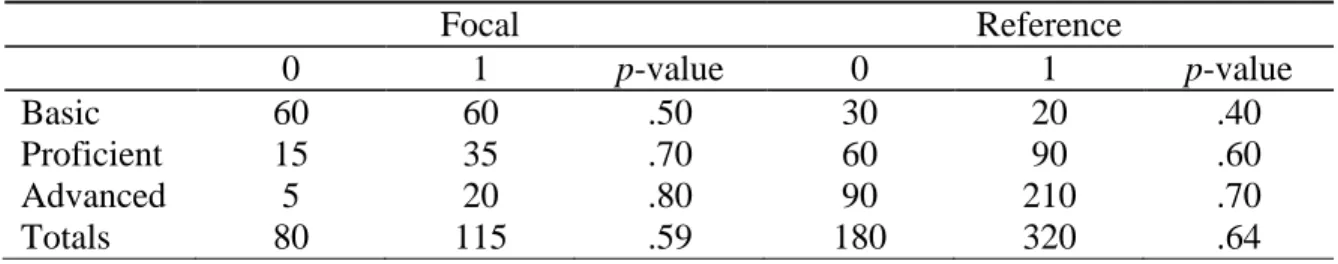
favor the other group. Table 1 provides a hypothetical illustration of Simpson’s Paradox. The table shows the performance of two groups, on one item, at three separate levels of ability.
Table 1: Simpson’s Paradox Example
Focal Reference
0 1 p-value 0 1 p-value
Basic 60 60 .50 30 20 .40
Proficient 15 35 .70 60 90 .60
An examination of the p-values shown in Table 1 reveals that, overall, the reference group has a 5% better chance of answering this item correctly (i.e., the p-value for the reference group is .64 versus .59 for the focal group). Paradoxically, however, the item favors the focal groupat each level of ability by 10%. Thus, for multiple reasons, simple
comparisons of p-values are no longer recommended for use in identifying DIF. More
modern methods that control for ability are based on item response theory (IRT) and
observed score methods such as logistic regression and chi-square tests. Observed score
methods are typically used with DIF studies involving small sample sizes (Camilli, 2006).
Item Response Theory
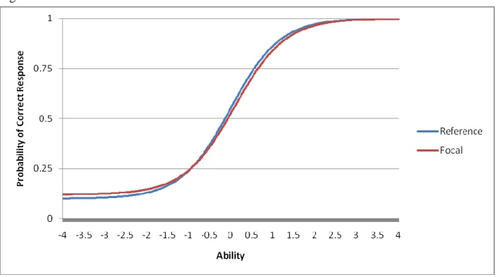
IRT involves using examinee’s responses and item characteristics to estimate an examinee’s ability via a one-, two-, or three-parameter logistic model. The estimates can then be compared across focal and reference groups (Camilli & Shepard, 1994). Once scores are standardized they can be displayed in an item characteristic curve (ICC), where the x-axis represents examinee ability level and the y-axis represents the probability of getting the item correct. If the ICCs of each group are equal, then construct-irrelevant variance is absent, or at least affects each group the same way. DIF exists if the ICCs of each group are different; in other words, examinees in the reference and focal groups of equal ability levels have differing probabilities of answering an item correctly (Crocker & Algina, 1986).
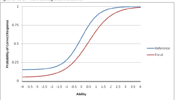
indicate that examinees in the reference and focal groups have differing probabilities of success on the item. An examinee in the focal group with an ability level of 0 has a probability of answering the item correctly of approximately .35. On the other hand, an examinee in the reference group with the exact same ability level has approximately a .50 chance of answering the item correctly.
Figure 2: ICCs with Differing Item Parameters
There are two approaches to identifying whether the ICCs of each group differ. The first method is to measure the differences (i.e. the effect size) between the ICCs of each group; the second method is to test the statistical significance of the group differences. Both approaches should be used in conjunction with each other because effect size differences may be due to chance and because statistically significant results due to large sample sizes may not have practical relevance (Camilli, 2006). An advantage of using IRT is its
capability of identifying both uniform and non-uniform DIF. Uniform DIF occurs when the ICCs of the reference and focal groups do not intersect. Conversely, non-uniform DIF occurs when the ICCs do intersect.
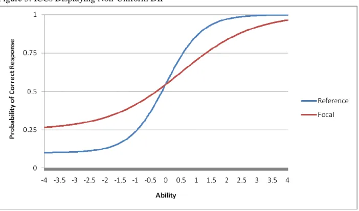
Figure 2 is an example of uniform DIF. The ICCs of the two groups are significantly different and they do not intersect. That means over the entire spectrum of ability the
non-of the ability distribution. At the lower end non-of the ability spectrum the item favors the focal group. Conversely, at the higher end of the ability spectrum the item favors the reference group.
Figure 3: ICCs Displaying Non-Uniform DIF
Logistic Regression
almost always statistically significant because unless an item is a misfit item, examinees with higher ability will have a greater probability of answering it correctly than examinees with lesser ability. One of the benefits of using logistic regression for DIF detection is its ability to identify both uniform and non-uniform DIF. If the group/ability interaction is significant, non-uniform DIF is present.
As is usual in statistical hypothesis testing, the logistic regression test statistic should be accompanied by a measure of effect size. The Zumbo-Thomas (1997) effect size measure requires a calculation of pseudo-R2 for two models. The first model is the base model where the independent variable is ability (total test score). The first model represents an absence of DIF. Group membership and the interaction between group and ability are introduced in the second model. The change in R2, ΔR2, between the two models is the effect size. If ΔR2 is at least 0.13 from the first to the second model, and the group membership variable is
statistically significant, then at least moderate DIF is detected. Jodoin and Gierl (2001) argued that the Zumbo-Thomas effect size measure was not sensitive enough and proposed that moderate DIF existed when ΔR2
is greater than 0.035 and the group membership variable is statistically significant.
The Mantel-Haenszel Chi-Square Procedure
goal was ―to reach the same conclusions in a retrospective study as would have been obtained from a forward (prospective) study‖ (p. 722).
The use of Mantel-Haenszel for indentifying DIF. Holland and Thayer (1988)
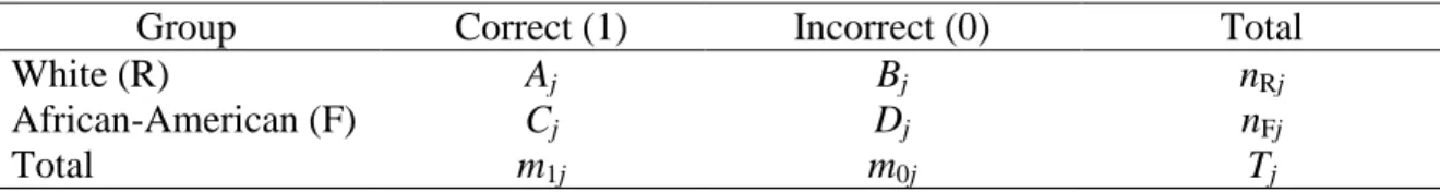
adapted the Mantel-Haenszel procedure for identifying DIF. The Mantel-Haenszel procedure
is essentially a 2 × 2 × J contingency table. The contents of the columns of the table represent whether the item was answered correctly or incorrectly, and the row contents
represent whether the examinees are members of the focal or reference groups. The focal
group, typically a minority group or other subgroup of interest, is the group being
investigated to determine whether its member’s responses to an item are an accurate
representation of their standings on a construct. The reference group, typically the majority
group, is the group which is being used as a standard for comparison to the focal group.
Examples of focal and reference groups could be male and female examinees, economically
disadvantaged and non-economically disadvantaged examinees, or Hispanic and Caucasian
examinees, respectively.
The J levels of the Mantel-Haenszel procedure – that is, the strata – should represent a measurement that allows for an effective comparison of the focal and reference groups. In educational testing, that measurement might represent total score on an end-of-grade
Table 2: Contingency table at score point J
Group Correct (1) Incorrect (0) Total
White (R) Aj Bj nRj
African-American (F) Cj Dj nFj
Total m1j m0j Tj
When conducting DIF analysis using the Mantel-Haenszel procedure, there would be a contingency table for each level of J for each item on the test. For instance, if there was a test with a maximum score point of 10 and a minimum score point of 5, for each item on the test there would be a contingency table at score points 5-10, assuming the full range of score points was achieved by the examinees.
Mantel-Haenszel test-statistic. The Mantel-Haenszel procedure requires a calculation of the following Chi-square test statistic:
(1)
where:
(2)
and
(3)
possessing the most statistical power for detecting departures from the null DIF hypothesis that are consistent with the constant odds ratio hypothesis‖ (p. 40). The Aj – E(Aj)
component of Equation 1 represents the difference between the actual number of correct responses for the item from the reference group for each ability level and the number of times the reference group would be expected to answer correctly, at the ability level j. If Aj > E(Aj), then it is possible the item displays DIF in favor of the reference group; whereas if Aj < E(Aj), then the item displays DIF favoring the focal group.
Mantel-Haenszel odds ratio. In addition to calculating the chi-square test statistic, the Mantel-Haenszel odds ratio provides a simple measure of effect size and is calculated with the following formula:
(4)
An odds ratio is the likelihood, or odds, of a reference group member correctly answering an item compared to a matched focal group member. The odds ratio can be difficult to interpret because items favoring the reference group range from 1 to infinity, while items favoring the focal group range from zero to one. To address this concern, Holland and Thayer (1988) suggested transforming the odds ratio by the natural logarithm so that the scores are centered around zero and easier to interpret. The range is subsequently transformed to negative infinity to positive infinity.
procedure to classify test items that display differing degrees of DIF by further transforming the natural log of the odds ratio by multiplying it by –2.35, yielding the ETS delta value:
|D| = –2.35*ln(αMH) (5)
According to Hambleton (2006), ―An ETS delta value represents item performance for a specified group of respondents reported on a normalized standard score scale for the construct measured by the test with a mean of 13 and a standard deviation of 4‖ (p. S184). After multiplying by –2.35, a positive delta value indicates the item favored the focal group whereas a negative delta value indicates the item favored the reference group. The categories are defined as:
Category A: Items display negligible DIF. |D| < 1.0 or MHX2 is not
significantly different than 0.
Category B: Items display intermediate DIF and may need to be reviewed for bias. MHX2 is significantly different than 0, |D| is > 1.0, and either |D| < 1.5 or
MHX2 is not significantly greater than 1.
Category C: Items display large DIF and are carefully reviewed for bias and possibly removed from the test. |D| > 1.5 and MHX2 is significantly different
than 1.
Benefits of using Mantel-Haenszel in DIF detection. In their research on the
accessibility, and inexpensiveness as benefits of the Mantel-Haenszel procedure. A Monte Carlo experiment conducted by Herrera and Gomez (2008) compared the Mantel-Haenszel procedure with logistic regression and found that uniform DIF detection rates were
significantly higher with Mantel-Haenszel when the reference and focal group sample sizes were relatively small (reference = 500; focal 500) or when the reference group was up to five times larger than the focal group. Small, unequal sample sizes are exactly the types of scenarios associated with DIF studies on test translations.
Research on the Mantel-Haenszel Procedure and Sample Size. Research has been
conducted on improving DIF detection when confronted with small sample sizes. Mazor et al. (1992) recommended that sample sizes should be at least 200 in each group, and their recommendation only referred to situations where DIF was most extreme. Van De Viljer (1997) noted that the Mantel-Haenszel procedure performs well when sample sizes for both the reference and focal groups are over 200. Parshall and Miller (1995) found that focal group sizes of at least 100 are needed to reach acceptable levels of DIF detection. Muniz et al. (2001) attempted to enhance the power of the Mantel-Haenszel procedure for small
sample sizes by combining certain score points into one score level to decrease the number of score level strata. However, their study was conducted with specific regard to situations where there are less than 100 cases; this technique is unnecessary when there are focal group sizes of at least 200, and research has shown that in general, more strata based on ability are better than fewer strata (Clauser, Mazor, Hambleton, 1994).
In their Monte Carlo study, Herrera and Gomez (2008) tested the influence of unequal sample sizes on the detection of DIF using the Mantel-Haenszel procedure. As the
the DIF detection rate decreased. In examples with unequal and small sample sizes (R = 500 and F = 100), the detection rate was 35%; however, when the distributions were equal (R = 500 and F = 500) the detection rate was 96%. Herrera and Gomez also reported that, with a reference group as large as 1,500 students, the focal group could be up to one fifth the size of the reference group without affecting the power of the Mantel-Haenszel procedure, at least under the circumstances of their experiment. They emphasized, however, that if the Mantel-Haenszel procedure is to be applied to unequal group sizes, the reference group should be greater than 1,500 cases and a focal group no more than five times smaller. Neither their research nor the vast majority of DIF research addresses a scenario where the reference group was 100 to 200 times larger than the focal group, as is likely to occur in a test translation DIF study of a high-stakes, statewide assessment.
Research on the Mantel-Haenszel Procedure and Ability Distribution
Differences. In addition to sample size differences, another factor affecting DIF analyses is the difference in the ability distributions of the reference and focal groups. The power of the Mantel-Haenszel statistic decreases as the ability distributions become more disparate (Herrera & Gomez, 2008; Mazor et al., 1992; Muniz et al., 2001; Narayanan &
compared, sample sizes of the focal group should be as large as possible, and even then DIF may not be correctly identified.
Using DIF for Translated Tests
A typical test translation in educational achievement testing is not likely to have more than a few hundred examinees (Fidalgo et al., 2004). IRT and logistic regression require more examinees to identify DIF effectively. Thus, of the three methods, the Mantel-Haenszel procedure would be the most effective for use in most test adaptations and other testing scenarios where there may be small sample sizes such as computer adaptive testing (CAT). However, there are caveats to this general conclusion. The statistical power of the Mantel-Haenszel procedure decreases as sample size decreases and as the ability
Propensity Score Matching
In certain situations it is not practical or ethical to conduct a clinical trial to appraise the effects of a treatment. In those situations, observational studies may be used to infer causal relationships. The same concept could be applied to educational experiments. For example, suppose a researcher was looking to assess the impact of charter schools versus traditional public schools on achievement. It would not be practical to conduct an
experiment in which students were randomly assigned to treatment (i.e., charter school) and control (i.e., traditional public school) groups, or to compare the achievement levels of the schools in question. Among other differences, charter schools have different selection processes than traditional public schools, and charter schools are not available in some areas around the country, amongst other differences. In such a situation, however, a researcher could use propensity score matching to control for differences between the two groups in variables such as: the selection process, geography, family participation, socio-economic status, and other variables deemed appropriate, in an effort to make a more valid assessment of the effects of the treatment (i.e., charter schooling).
A propensity score can be conceptualized as the probability of receiving the treatment condition in an experiment. Propensity scores may be estimated with various methods including logistic regression, a probit model, and discriminant analysis. According to Guo and Fraser (2010), logistic regression is the dominant method for estimating propensity scores and thus was the approach used for this thesis.
to Parsons (2001), there are basically two types of matching algorithms: greedy matching and
optimal matching.
Greedy Matching. Greedy matching involves matching one case from the treatment
group to a case from the non-treatment group with the most similar propensity score. The match that is made for any given case is always the best available match and once that match has been made it cannot be reversed. According to Guo and Fraser (2010) greedy matching requires a sizable common support region for it to work properly. The common support region is defined as the area of the two distributions of propensity scores where propensity scores overlap. The cases from each the focal and reference groups that are outside of the common support region are not matched and subsequently eliminated from analysis. Then, the greedy algorithm is used to match the propensity score of one case from the treatment group to one case in the control group. Identification of the rest of the matches will follow the same procedure.
Optimal Matching. As computers have become faster and software packages more
matching thus minimizes the distance between matches.
The Importance of DIF Detection for Translated Items
Why is detecting DIF in test translations and adaptations of crucial importance? There is very little research on why test items in one language measure differently than the same items in another language (Allalouf et al., 1999). One of the hypothesized reasons for the lack of research is that there are limited methods for assessing DIF in the scenarios associated with test translations. The reasons translated items measure differently for
populations taking a test in different languages need to be better understood. Test developers could use the greater understanding of why DIF occurs in test translations to improve
guidelines for item writing. Furthermore, items that would eventually be translated to another language could be improved earlier in the test adaptation process. For example, previous research has shown that translated analogy items display more DIF than sentence completion or reading comprehension items (Angoff & Cook, 1988; Beller, 1995). In
research done on the Israeli university entrance exam, the Psychometric Entrance Test (PET), Allalouf et al. (1999) noted four possible reasons why translated items performed differently for Russian or Hebrew language examinees: 1) changes in difficulty of words or sentences, 2) changes in content, 3) changes in format, and 4) differences in cultural relevance. The analogy items displayed DIF more regularly than the other item types mainly due to changes in word difficulty or changes in content. For instance, in Hebrew there are more difficult synonyms or antonyms to choose from than in Russian. Thus, an analogy question in Hebrew might be very challenging, but the same item might be relatively easy when translated into Russian.
accurate methods were developed for identifying items that were measuring differently for each sub-group of examinees, then linking the two test forms (i.e. the original and translated) could be performed with greater accuracy. Sireci (1997) recommended that the linking process should begin with an evaluation of the translated test items for invariance between the two tests, and items displaying DIF should be removed. The remaining items not displaying DIF could then be used as anchors, and the two tests calibrated onto a common scale. However, if the methods for identifying DIF misidentify items that are functioning differently for different sets of examinees, then the linking process will not be as accurate as possible.
Summary
Of all the techniques used to evaluate DIF, the Mantel-Haenszel procedure is the most effective with small sample sizes. Thus, it is optimal for use in evaluating DIF in a typical test translation where there are only a few hundred examinees. However, the ability distributions and the total numbers of examinees are often vastly different when comparing the population of examinees who received the translated version of the test against the general population of examinees. The accuracy of the Mantel-Haenszel procedure decreases as the ability distributions and the total population of examinees become more disparate. Propensity score matching can be used to control for the distributional differences between the two populations, possibly enhancing the Mantel-Haenszel procedure for identifying DIF. If items that are measuring differently for the two populations can be more accurately
Research Question
Method
This study used simulated data to provide a known benchmark against which the performance of PSM was evaluated. The data for this study were generated using the program WinGen2 (Han, 2007). The program simulates examinee responses using the type of IRT model specified by the user. WinGen2 also allows for DIF to be introduced into the examinee responses. For this study the Rasch model was used because the item parameters and ability levels of the reference and focal groups were based off of data that was calibrated with the Rasch model. The Rasch model is commonly used to analyze data in large-scale, statewide assessments. The data were simulated to resemble a standard administration of a statewide assessment that was delivered in two versions; in this case, to simulate
administrations of English and Spanish versions. Each data set was simulated with a test length of 50 items—a test length that would not be unrealistic for a statewide student achievement test.
Variables in Study
Three primary independent variables were manipulated in this study. The variables included sample size, ability distributions, and amount of DIF.
Sample Size. One data set of 100,000 examinees was simulated to represent the
reference group. Three other data sets of 250, 500, and 1,000 were simulated to represent the focal groups.
at –0.30 with a standard deviation of approximately 0.65. The ability distributions were simulated to resemble a standard administration of a statewide assessment that was delivered in both English and Spanish. Experience suggests that the population of examinees who received the Spanish accommodation to test in their native language had significantly lower ability levels than the English population. The Spanish population’s average ability level was approximately 1.3 standard deviations lower than the average ability level of the English population.
Amount of DIF. Experience with translated language testing suggests that DIF is
likely to be observed in approximately 25-40% of translated test items. Therefore, 16 of the 50 items (32%) had DIF introduced to their item difficulty parameters. The 16 items were selected to be representative of the test as a whole, meaning the range, mean, and standard deviation of the DIF subtest is similar to the whole test. To increase the generalizability of the study and because DIF occurs at different levels depending on the test translation, DIF was introduced in two scenarios in four increments at each level: 0.2, 0.4, 0.6, and 0.8 in the first scenario and 1.0, 1.2, 1.4, and 1.6 in the second scenario. A DIF level of 1.0 would mean that the item-difficulty parameter of the focal group had been increased by 1.0. For instance, item #34 had an item-difficulty parameter of -1.014. A DIF level of 1.0 was added and the item-difficulty for the focal group changed from -1.014 to -0.014. To introduce DIF in favor of the focal group the DIF level would be subtracted from the item-difficulty
taken place, DIF levels of 1.5 or higher are not uncommon. The first scenario represents a test with moderate levels of DIF, and the second scenario represents a test with large levels of DIF. Experience suggests DIF favors the reference group approximately 75% of the time and the focal group approximately 25% of the time. Thus, 12 of the items have DIF in favor of the reference group and 4 in favor the focal group. Table A1 in Appendix A shows the item difficulty parameters for all 50 items as well as the introduction of DIF for each scenario.
Data Analyses
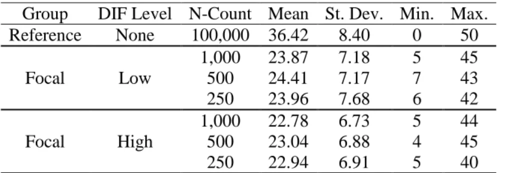
For each simulation condition, descriptive statistics were calculated including p -values, response variance, and point-biserial correlations for each item. Reliability estimates were calculated using Cronbach’s Alpha. The descriptive statistics and reliability estimates were analyzed to ensure the simulated data resembled a typical administration of high-stakes statewide assessment. All descriptive statistics and reliability estimates were calculated using a SAS computer program written by the author. The SAS code used for this thesis is in Appendix B. Table 3 displays the total test score mean and standard deviation, as well as the range of scores for all seven simulated data sets.
Table 3: Total Test Score Descriptive Statistics for Simulated Data Sets Group DIF Level N-Count Mean St. Dev. Min. Max. Reference None 100,000 36.42 8.40 0 50
Focal Low
1,000 23.87 7.18 5 45
500 24.41 7.17 7 43
250 23.96 7.68 6 42
Focal High
1,000 22.78 6.73 5 44
500 23.04 6.88 4 45
The Mantel-Haenszel procedure was applied to the entire population of simulated examinees using a SAS computer program written by the author. The reference group represented the population of examinees who took the test in the language in which the test was originally written. The focal group represented the population of examinees who took the translated version of the test. The results reported in the next section tested the
significance level of the Mantel-Haenszel test statistic at the .05 level. Items were also classified using the classification system proposed by Dorans and Holland (1993).
Propensity Score Matching. After verifying the simulation conditions were met via
the generated data and classifying each item with the traditional Mantel-Haenszel procedure, an estimated propensity score was calculated for each case in both the reference and focal groups for all simulation scenarios. The propensity score was based on total test score. After obtaining the estimated propensity scores, greedy matching was used to accomplish the matching. Greedy matching requires less computing power and programming than optimal matching (Guo and Fraser, 2010). Because there was such a large pool of simulated
reference examinees compared to the relatively small groups of simulated focal examinees, and because only one variable (total score) was used for matching, it was unlikely that matching via greedy matching or optimal matching would produce significantly different matches. Furthermore, the two populations had a large common support region of propensity scores, meaning the major assumption of greedy matching was satisfied (Parsons, 2001; Rosenbaum, 2002). The greedy matching was performed with a variation of Parsons’ (2001) greedy matching macro using SAS software.
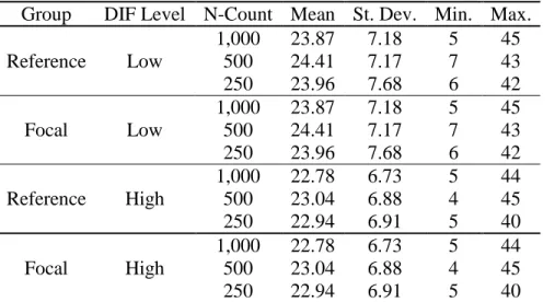
examinees in the reference group, and because matching was accomplished via total test score, the means and standard deviations for each group were equal after matching. Table 4 shows the descriptive statistics of all groups after matching.
Table 4: Total Test Score Descriptive Statistics for Simulated Data Sets After Matching Group DIF Level N-Count Mean St. Dev. Min. Max.
Reference Low
1,000 23.87 7.18 5 45
500 24.41 7.17 7 43
250 23.96 7.68 6 42
Focal Low
1,000 23.87 7.18 5 45
500 24.41 7.17 7 43
250 23.96 7.68 6 42
Reference High
1,000 22.78 6.73 5 44
500 23.04 6.88 4 45
250 22.94 6.91 5 40
Focal High
1,000 22.78 6.73 5 44
500 23.04 6.88 4 45
250 22.94 6.91 5 40
differences in Type I and II errors were statistically significant, or if any of the interactions between method, sample size, and DIF level were statistically significant.
Summary
The purpose of this thesis is to answer the following research questions:
1) What is the effect on the Type I errors of the Mantel-Haenszel procedure in assessing DIF when propensity score matching is used to control for distributional differences between the reference and focal groups?
2) What is the effect on the Type II errors of the Mantel-Haenszel procedure in assessing DIF when propensity score matching is used to control for distributional differences between the reference and focal groups?
3) What are the effects of focal group sample size, the level of DIF and the method of DIF detection (e.g. with or without matching) on Type I errors.
4) What are the effects of focal group sample size, the level of DIF and the method of DIF detection (e.g. with or without matching) on Type II errors.
5) What is the effect on the ETS classifications of the Mantel-Haenszel procedure in assessing DIF when propensity score matching is used to control for distributional differences between the reference and focal groups?
To address research question 1 a repeated measures ANOVA was conducted with Type I errors for each method of DIF detection as the dependent variable and sample size and DIF level as the independent variables. To address research question 2 another repeated measures ANOVA was conducted. In this case, Type II errors for each method of DIF detection was used as the dependent variable and sample size and DIF level were the
Results
The first component of the results section addresses the simulated data. Do the simulated data resemble a standard administration of a Language Arts Literacy high-stakes statewide assessment that was delivered in both English and Spanish? P-values, point-biserial correlations, and Cronbach’s alpha were calculated and analyzed to answer that question. The next components of the results section will address each of the research questions in the order they were presented in the methods section and the subsequent results of the study.
Simulated Data
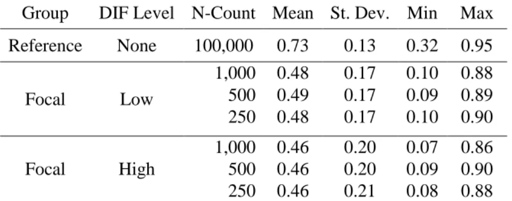
As previously stated, the p-values were calculated to ensure the data sets adequately resembled a standard administration of a Language Arts Literacy high-stakes statewide assessment that was delivered in both English and Spanish. Table 5 summarizes the item difficulty descriptive statistics for reference and focal groups, at each combination of DIF level and focal group size. Based on prior experience, the summary of item difficulties in Table 5 for each of the seven data sets does not appear unrealistic. Tables C1-C6 are found in Appendix C. They display the p-values for each item for all six cells of the study’s design, before and after matching. Tables C1-C6 also display the item variances for each of the six scenarios, before and after matching. The item variances tended to be larger with the focal group population than with the reference group. Considering the average p-values in Table 5 the larger item variances associated with the focal groups are not surprising. Items with
reference group was 0.73 compared to average focal group p-values that were much closer to 0.5.
Table 5: Descriptive Statistics of Item Difficulties of Simulated Data Sets Group DIF Level N-Count Mean St. Dev. Min Max
Reference None 100,000 0.73 0.13 0.32 0.95 Focal Low
1,000 0.48 0.17 0.10 0.88 500 0.49 0.17 0.09 0.89 250 0.48 0.17 0.10 0.90 Focal High
1,000 0.46 0.20 0.07 0.86 500 0.46 0.20 0.09 0.90 250 0.46 0.21 0.08 0.88
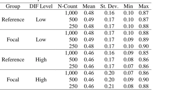
Table 6 summarizes the item difficulty descriptive statistics after matching at each combination of DIF Level and focal group size. The average p-value of the reference group went from 0.73 to ranging from 0.46 to 0.49, depending on which focal group data set it was matched to. The matched reference groups’ average p-values are equivalent to the p-values of their associated focal group. There are slight differences between the standard deviations of the matched reference groups and the focal groups, as well as the minimum and maximum
Table 6: Descriptive Statistics of Item Difficulties of Simulated Data Sets Post-Matching Group DIF Level N-Count Mean St. Dev. Min Max
Reference Low
1,000 0.48 0.16 0.10 0.87 500 0.49 0.17 0.10 0.87 250 0.48 0.17 0.10 0.88
Focal Low
1,000 0.48 0.17 0.10 0.88 500 0.49 0.17 0.09 0.89 250 0.48 0.17 0.10 0.90 Reference High
1,000 0.46 0.16 0.09 0.85 500 0.46 0.17 0.08 0.86 250 0.46 0.17 0.07 0.86
Focal High
1,000 0.46 0.20 0.07 0.86 500 0.46 0.20 0.09 0.90 250 0.46 0.21 0.08 0.88
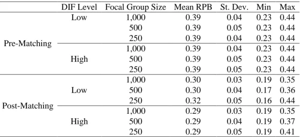
Table 7: Descriptive Statistics of Point-Biserial Correlation: Pre and Post-Matching DIF Level Focal Group Size Mean RPB St. Dev. Min Max
Pre-Matching
Low 1,000 0.39 0.04 0.23 0.44
500 0.39 0.05 0.23 0.44
250 0.39 0.04 0.23 0.44
High
1,000 0.39 0.04 0.23 0.44
500 0.39 0.05 0.23 0.44
250 0.39 0.05 0.23 0.44
Post-Matching
Low
1,000 0.30 0.03 0.19 0.35
500 0.30 0.04 0.17 0.36
250 0.32 0.05 0.16 0.44
High
1,000 0.29 0.03 0.19 0.35
500 0.29 0.04 0.19 0.37
250 0.29 0.05 0.19 0.41
Cronbach’s Alpha values were calculated for the reference group and all six focal groups to ensure the simulated data accurately resembled a typical administration of high-stakes statewide assessment. Table 8 displays the reliability estimates and standard errors of measurement of the simulated data. Based on experience with high-stakes statewide
assessments delivered in both English and Spanish, the reliability estimates and standard errors of measurement measures in Table 8 do not appear unrealistic.
Table 8: Summary of Cronbach’s Alpha Reliability Estimates and SEMs for each Simulated Data Set
Group DIF Level N-Count Alpha SEM Reference None 100,000 0.89 2.80
Focal Low
1,000 0.80 3.20 500 0.80 3.20 250 0.83 3.18 Focal High
Type I Errors
Table 9 displays the contingency table of total Type I errors for both pre- and post-matching. Only the 34 items where DIF was not introduced were considered in determining the Type I error rate. Because there were six possible scenarios representing each
combination of the two levels of DIF and the three sample sizes, and 34 items per scenario that had the potential for Type I errors, there were 204 total repeated measures that were used in the contingency table shown in Table 9. One finding is the large number of Type I errors pre-matching. Approximately 30% of items (61 out of 204) were classified as showing statistically significant DIF, when no DIF had been introduced. Matching decreased the percentage of Type I errors to 18% (36 out of 204). The results of the repeated-measures ANOVA (Wilk’s Lambda = .91, F(1,198) = 19.04, p < 0.0001) suggest that the decrease in Type I errors was statistically significant. Matching is having a positive effect on decreasing Type I error rates and thus the null hypothesis -- that matching is having no effect on the Type I error rate of the Mantel-Haenszel procedure -- is rejected.
Table 9: Contingency Table for Type I Errors
Post-Matching
Type I Error No Yes Total Pre-Matching
No 136 7 143
Yes 32 29 61
Total 168 36 204
out of 102) pre-matching and to 26% (27 out of 102) post-matching. Table 10 suggests that the statistically significant decrease in Type I errors after matching is largely due to the interaction between the method of identifying DIF and the DIF level. The interactions between the method of identifying DIF, sample size, and DIF level in Type I errors will be discussed further in a section below.
Table 10: Total Number of Type I Errors
DIF Level Focal Group Size Type I Errors
Pre-Matching
Low
1,000 5
500 2
250 2
High
1,000 28
500 13
250 11
Post-Matching
Low
1,000 4
500 2
250 3
High
1,000 15
500 7
250 5
Type II Errors
hypothesis -- that matching is having no effect on the Type II error rate of the Mantel-Haenszel procedure -- is rejected.
Table 11: Contingency Table for Type II Errors
Post-Matching
Type II Error No Yes Total Pre-Matching
No 83 6 89
Yes 1 6 7
Total 84 12 96
Table 12 displays the total number of Type II errors both pre-and post-matching for each combination of sample size and DIF level. One major finding is that when the DIF level was high, neither method produced a Type II error. Regardless of samples size, all 16 items that had a high level DIF introduced were correctly identified as displaying DIF regardless of method. Another, less encouraging finding is the number of Type II errors found when the DIF level was low. Pre-matching and with low levels of DIF, the percentage of Type II errors was 15% (7 out of 48) and post-matching it increased to 25% (12 out of 48).
Table 12: Total Number of Type II Errors
DIF Level Focal Group Size Type II Errors
Pre-Matching
Low
1,000 2
500 2
250 3
High
1,000 0
500 0
250 0
Post-Matching
Low
1,000 3
500 2
250 7
High
1,000 0
500 0
Effects on Type I Errors
The repeated-measures ANOVA was also conducted to answer research question #3 and determine the effect of the DIF methodology, sample size, and DIF level, as well as the interactions between those three variables on Type I errors. Table 13 displays the results of the ANOVA on Type I errors. All three main effects were found to be statistically
significant: method [F(1,198) = 19.04, p <0.0001], sample size [F(2, 198) = 10.95, p
<0.0001], and DIF level [F(1, 198) = 46.46, p <0.0001]. The fact that method is a
statistically significant main effect suggests that the methodology chosen (i.e. matching or no matching) is having a statistically significant effect on Type I errors. Furthermore, that the main effects of sample size and DIF level are also statistically significant indicates that as sample size or the level of DIF increases then an increase in Type I errors can be expected, regardless whether matching is used to control for ability distributions or not. Two of the interactions were statistically significant: method x DIF level [F(1, 198) = 19.04, p = .001] and sample size x DIF level [F(1, 198) = 5.48, p = .0048]. These findings suggest that the interaction between methodology and DIF level is significant and that the impact of one factor depends on the level of the other. Thus, any interpretation of the statistical significance of the methodology without noting the interaction between DIF level and
Table 13: Analysis of Variance for Type I Errors
Source df F p
Method 1 19.04 <0.0001
Sample Size 2 10.95 <0.0001
DIF Level 1 46.46 <0.0001
Method x Sample Size 2 2.22 0.1108
Method x DIF Level 1 19.04 <0.0001 Sample Size x DIF Level 2 5.48 0.0048 Method x Sample Size x DIF Level 2 0.94 0.3906
Effects on Type II Errors
A repeated-measures ANOVA was also conducted to answer research question #4 and determine the effect of the DIF methodology, sample size, and DIF level, as well as the interactions between those three variables on Type II errors. Table 14 displays the results of the ANOVA on Type II errors. In Table 14 only two main effects had a statistically
significant impact on Type II errors: method [F(1,90) = 3.95, p =0.05] and DIF level [F(1,90) = 15.25, p = 0.0002]. Sample size [F(2, 90) = 1.31, p = 0.275] was not statistically
significant. The results in Table 14 suggest that the methodology chosen is making a statistically significant impact on Type II errors. Method x DIF level [F(1,90) = 3.95, p
=0.05] was the only statistically significant interaction.
Table 14: Analysis of Variance for Type II Errors
Source df F p
Method 1 3.95 0.0500
Sample Size 2 1.31 0.2750
DIF Level 1 15.25 0.0002
Method x Sample Size 2 2.05 0.1344
Method x DIF Level 1 3.95 0.0500
ETS Classification Agreement Rates
Because statistically significant results are not always of practical importance, the ETS classifications of each of the methods were calculated and analyzed. Table 15 displays the number of items that were classified as either A, B, or C by the ETS classification system, at all combinations of DIF level and sample size, both before and after matching. One finding of Table 15 is that both methods produced very similar distributions of
classifications. The distributions of classifications were exactly the same for both methods when the DIF level was low and sample size was 250 as well as when the DIF level was high and sample size was 1,000. A second finding is that both methods appeared to be under classifying DIF items when the DIF level was low, regardless of sample size. Of the 16 items where DIF was introduced, only 8 to 10 items were flagged as B or C items when the DIF level was low. Furthermore, when the DIF level was high and samples sizes were 500 or 250, more items were classified as displaying DIF than the 16 items that had DIF
introduced. Tables C1-C6 in Appendix C display the ETS classifications, before and after matching, for each item at all combinations of DIF level and sample size.
Table 15: Distribution of A, B, & C Class items for both Pre- and Post-Matching Degree of DIF
DIF Level Focal Group Size A B C
Pre-Matching
Low 1,000 41 4 5
500 42 7 1
250 40 8 2
High
1,000 34 0 16
500 34 0 16
250 31 3 16
Post-Matching
Low
1,000 42 3 5
500 42 6 2
250 40 8 2
High
1,000 34 0 16
Tables 16-21 display the contingency tables for the ETS classification system as well as the agreement rate and Cohen’s Kappa for each of the six combinations of sample size and DIF level. The agreement rates were all over 92%. When the sample size was 1,000 and the DIF level was high the agreement rate of the two methods was 100%. Cohen’s Kappa statistics ranged from 0.76 to 1.00. According to Landis and Koch (1977) a Kappa statistic between 0.61 and 0.80 indicates substantial agreement and between 0.81 and 1.00 indicates almost perfect agreement. The high agreement rates and the large Kappa statistics suggest that controlling for distributional differences is having a limited affect on the ETS
classification of items.
Table 16: ETS Classification Contingency Table – Sample Size = 1000; DIF Level = Low Post-Matching
ETS Class. A B C Total Pre-Matching
A 41 0 0 41
B 1 3 0 4
C 0 0 5 5
Total 42 3 5 50
Agreement Rate = 98% Cohen’s Kappa = 0.93 (p < .0001)
Table 17: ETS Classification Contingency Table – Sample Size = 500; DIF Level = Low Post-Matching
ETS Class. A B C Total Pre-Matching
A 41 1 0 42
B 1 5 1 7
C 0 0 1 1
Total 42 6 2 50
Table 18: ETS Classification Contingency Table – Sample Size = 250; DIF Level = Low Post-Matching
ETS Class. A B C Total Pre-Matching
A 38 2 0 40
B 2 6 0 8
C 0 0 2 2
Total 40 8 2 50
Agreement Rate = 92% Cohen’s Kappa = 0.76 (p < .0001)
Table 19: ETS Classification Contingency Table – Sample Size = 1000; DIF Level = High Post-Matching
ETS Class. A B C Total Pre-Matching
A 34 0 0 34
B 0 0 0 0
C 0 0 16 16
Total 34 0 16 50
Agreement Rate = 100% Cohen’s Kappa = 1.00 (p = N/A)
Table 20: ETS Classification Contingency Table – Sample Size = 500; DIF Level = High Post-Matching
ETS Class. A B C Total Pre-Matching
A 31 3 0 34
B 0 0 0 0
C 0 0 16 16
Total 31 3 16 50
Agreement Rate = 94% Cohen’s Kappa = N/A
Table 21: ETS Classification Contingency Table – Sample Size = 250; DIF Level = High Post-Matching
ETS Class. A B C Total Pre-Matching
A 28 3 0 31
B 0 3 0 3
C 0 1 15 16
Discussion
This section is organized around three major topics. The first topic of interest is the implications of the findings of this study: What has been learned and why is it important? The second topic of interest is the limitations of the study; no study is perfect and by
understanding the limitations of this study a greater understanding of the topic in general can be established. Finally, the avenues for future research are discussed: What are some next steps in researching identification of DIF in the context of test translations?
Implications of Findings
The focus of this study was to test the effects of controlling for disparate
distributional differences on the Mantel-Haenszel procedure. Would controlling for those differences increase its ability to detect DIF accurately? To answer that question a repeated-measures ANOVA was conducted to test the main effects of DIF methodology (pre-matching Mantel-Haenszel or post-matching Mantel-Haenszel), focal group sample size (1,000, 500, or 250) and DIF level (low or high). The interactions between those three variables were also tested. Finally, the ETS classifications of each item, using each methodology were analyzed. The findings suggest that Type I errors of the Mantel-Haenszel test statistic can be decreased by matching. However, there is a caveat to that finding. The error rate in the ETS
classification of items increased after matching.
Type I Errors. If DIF researchers identify DIF where no DIF exists then valuable
Research question #1 asked whether matching was having an effect on the Type I error rates. The statistically significant decrease in Type I errors after matching the ability distributions of the focal and reference groups is a positive finding. However, it was expected that matching would result in a statistically significant decrease in the Type I errors made in the Mantel-Haenszel procedure. As sample size increases, Type I errors should increase as well: Any test statistic will become more powerful as sample size increases. The statistically significant decrease in Type I errors should only be interpreted in conjunction with an effect size measure such as the ETS classification system, which will be discussed when research question #5 is addressed.
Type II Errors. Just as DIF researchers look to avoid analyzing items for bias that actually have no DIF, they want items that are biased to be identified as displaying DIF so that the source of that bias may be investigated. Research question #2 asked whether matching was having an effect on the Type II errors rates. There was a statistically
significant difference in Type II errors between the Mantel-Haenszel procedure before and after matching. In this case, the statistically significant results were not in favor of the Mantel-Haenszel procedure after matching. Thus, the decrease in sample sizes after matching is decreasing the power of the Mantel-Haenszel procedure enough that it
Effects on Type I Errors. Research question #3 addressed the effects of focal group sample size, the level of DIF and the method of DIF detection (e.g. with or without
matching) on Type I errors. The main effects of sample size, DIF level and method were all determined to be statistically significant, as well as two two-way interactions: method–by-DIF level as well as sample size–by-method–by-DIF level. That method was statistically significant gives more credence to the argument that matching could decrease Type I errors rates. That sample size is statistically significant should be of no surprise. As was discussed earlier, as sample size increases, power increases, and Type I error rates increase. Furthermore, that DIF level was statistically significant should not have been surprising. The higher the DIF level the more likely pseudo-DIF will become prevalent in other items. Psuedo-DIF is when true-DIF in one item causes apparent DIF in other items within the same test, even though these other items are not truly differentially functioning (Groenvold & Petersen, 2005). Thus, items without DIF may display pseudo-DIF to compensate for items that actually display true-DIF. As DIF levels increase, pseudo-DIF increases which might account for the statistically significant impact of DIF level on Type I errors.
classroom B might have got the biased correction incorrect and still got a 26. The extra point student B earned would have had to come from somewhere else on the test, on an item that was not biased. If the extra points earned by focal group examinees to compensate for the true-DIF accumulate in enough frequency on one or two items, pseudo-DIF might get large enough to be statistically significant. The more extreme the DIF, and the less points that are available in the total test score, the more pseudo-DIF will be a problem, unless the internal scale is purified as recommended by Clauser, Mazor, and Hambleton (1993).
Figure 4: Interaction of DIF Level and Method in Type I Errors
0 2 4 6 8 10 12 14 16 18 20
Low High
DIF Level
Ty
pe
I
E
rr
ors
Pre-Matching
Post-Matching
Effects on Type II Errors. Research question #4 addressed the effects of focal
group sample size, the level of DIF and the method of DIF detection (e.g. with or without matching) on Type II errors. Only the main effects of method and DIF level were deemed statistically significant. That DIF level was statistically significant was not surprising. When the DIF level was lower, it was more challenging for the Mantel-Haenszel procedure to detect DIF.
post-matching was 4. Using pre-post-matching, it was only 2.33. The implications of these findings are that if researchers are anticipating doing DIF analyses on a test with possible low levels of DIF, matching could increase Type II errors. However, if researchers are performing DIF analysis on a test with anticipated high levels of DIF, such as a test translation, pre-matching and post-matching will likely produce similar Type II error rates. However, those findings should only be interpreted in conjunction with a measure of effect size, such as the ETS classification system.
Figure 5: Interaction of DIF Level and Method in Type II Errors
0 0.5 1 1.5 2 2.5 3 3.5 4 4.5
Low High
DIF Level
Ty
pe
I
I
E
rr
ors
Pre-Matching
Post-Matching
ETS Classification Agreement Rates. Just looking at Type I or II errors is not a
complete analysis. Effect size measures such as the Mantel-Haenszel log odds ratio, a