Verification of micro-scale photogrammetry for
smooth three-dimensional object measurement
Danny Sims-Waterhouse, Samanta Piano and Richard Leach
Manufacturing Metrology Team, University of Nottingham
E-mail: [email protected]
Abstract.
1. Introduction
Photogrammetry is a passive triangulation technique based on the matching of points between many images of an object [1]. Through the matching of points over the surface of an object, photogrammetry is able to triangulate a point cloud for which geometric information about the object may be extracted. The accuracy and working range of photogrammetry depend on many factors, the most important of which are the camera parameters and reconstruction algorithms. Given the significant advancements of both imaging and computation technologies over the last few decades, photogrammetry has been able to extend its range down to sub-millimetre scales. Commercial systems, such as the geodetic V-STARS range, are already able to measure objects 1 m to 10 m in size with uncertainties of 5 µm + 5µm/m [2]. In particular, more recent research has shown that photogrammetry has the potential to provide three-dimensional (3D) form measurements to standard uncertainties of less than 10 µm [3–9]. There are other applications of photogrammetry able to produce even lower uncertainties, such as reconstructions based on scanning electron microscope (SEM) images [10]. Although SEM based photogrammetry is able to produce high magnification images, it will not be covered by the scope of this paper due to other issues such as cost, field of view and surface pre-processing. Given the relatively low uncertainties of recent results, photogrammetry is promising for micro-scale coordinate metrology.
The production of miniature, complex, high-precision components is key to the transition to high-value manufacturing [11]. There are a range of techniques able to measure 3D features at the micro-scale level, each of which is subject to some limitations [12]. Stylus instruments and micro-coordinate measuring machines are able to measure the form of objects to low uncertainties by placing a mechanical tip in contact with the object surface and monitoring the response. However, for highly complex parts, contact instruments can take many hours to produce a sufficiently dense grid of points. Optical techniques are able to measure millions of points within a single measurement, greatly reducing the time required to measure complex geometries. Although optical techniques, such as laser triangulation and micro-fringe projection, provide similar reductions in operation time, photogrammetry has significant benefits. The simplicity of photogrammetry means that system costs can be substantially lower than other micro-scale geometry measurement techniques and is a very simple technique in practice. Overall, photogrammetry provides a simple, low-cost technique for the measurement of highly complex surface geometries.
detection methods becomes problematic. Manufacturing sub-millimetre targets is both expensive and complex, and the target itself can distort the geometry of the artefact.
Photogrammetry methods for objects without targets are reliant on the process of feature detection and matching. Scale invariant feature transform (SIFT) algorithms are widely regarded as the most effective method of feature detection [17], and are based on the detection of local minima and maxima within a difference-of-Gaussian function. Detected features can then be matched by assigning unique descriptors based on local gradients and directions of the difference-of-Gaussian function [18]. In order for SIFT algorithms to detect any features, there must be some variation within neighboring pixels, which is observed as texture in the image, for this reason, objects with very little surface texture will not exhibit enough features for SIFT algorithms to detect. Although this inability to detect objects with little texture is an intrinsic limitation of photogrammetry, it is particularly problematic when considering the verification of a photogrammetry system. As will be discussed in Section 2.2, verification artefacts are required to have surface height variation values significantly smaller than the anticipated measurement uncertainty. This means that for a photogrammetry system to be verified to a standard uncertainty of the order of a few micrometres, an artefact with a surface height variations less than 1 µm is required. An object with such a smooth surface would not display any surface texture detectable by the system and as a result, will cause it to fail.
2. Methodology
2.1. System design
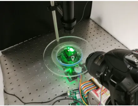
[image:4.612.184.404.421.590.2]The photogrammetry system can be seen in Figure 1. The system consists of a simple rotating stage and camera mount that allows the desired number of images to be taken at a range of angles. The positions of the camera can also be altered in order to produce the required image magnification at a range of camera elevation angles. The imaging system itself consists of a commercial DSLR camera (Nikon D3300, 24 MP sensor) with a 60 mm macro lens to allow high magnification images. The laser speckle system is mounted directly to the rotating table to ensure that the speckle pattern remains stationary with respect to the object as it rotates. Tests were also performed to ensure the projected pattern remained stable over one hour period, much longer than the time required for any particular experiment. Both the average and standard deviation of all SIFT features were monitored for the length of the test relative to the first image. The average motion was around two to three pixels, and corresponds to the mechanical stability of the camera. Despite the camera motion, for the duration of the test the calculated standard deviation of the average motion was less then one pixel, corresponding to the relative motion of the speckle features on the object surface. Since the variation of the pattern is less than one pixel, we are confident that the pattern will remain stable for the duration of the measurements.
Figure 1. Image of the photogrammetry system, rotation stage and speckle pattern.
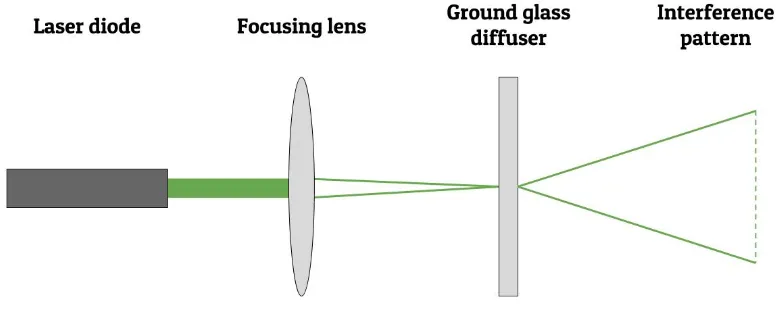
matched by SIFT algorithms. A significant requirement for the laser speckle system is that the object surface diffusely reflects the speckle pattern in order for the pattern to be observed on the objects surface. There will also be some further interaction of the laser speckle pattern with the object surface, creating subjective speckle. Subjective speckle is an unwanted pattern as it will vary depending on the camera position, and therefore, will not produce corresponding features [22]. However, by selecting a sufficiently low F-stop value (F/8), the contrast of the subjective speckle can be reduced to become effectively zero.
Figure 2. Schematic design of the laser speckle projection system.
2.2. Current specification standards
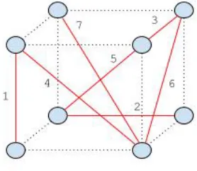
Figure 3. Seven ball bar orientations as defined by VDI/VDE 2634 part 3.
2.3. Artefacts
As we have seen in Section 2.2, a sphere and ball bar are required for the verification of a photogrammetry system according to VDI/VDE 2634 part 3. Therefore, one 10 mm diameter and three 5 mm diameter tungsten carbide tooling balls were selected to construct the required artefacts [23]. The tungsten carbide tooling balls have a roundness of 0.2 µm and an Ra parameter of 0.25 µm, whilst still having a diffusely reflecting surface ideal for photogrammetry [24, 25]. The 10 mm sphere was used as the probing error measurement sphere and placed in an object holder for individual use. The three 5 mm spheres were used to construct a ball plate, the design of which can be seen in Figure 4. The triangular orientation of spheres in Figure 4 was chosen such that three individual ball bar lengths could be measured from a single measurement. The ball bar lengths were calibrated using a Ziess F25 coordinate measurement machine (CMM) with a maximum permissible error of 0.25 µm [26]. After calibration, the 6 mm, 8 mm and 10 mm lengths were found to be 5.942 µm, 7.956 µm and 9.957µm respectively.
[image:6.612.154.441.531.662.2]2.4. Modified tests
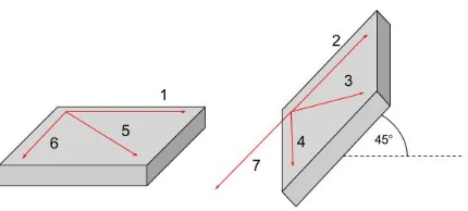
[image:7.612.186.401.308.405.2]The probing form and size error tests can be performed exactly as described in VDI/VDE 2634 part 3. However, replicating the ball bar arrangements in Figure 3 proves problematic when including the laser speckle projection system. As can be seen in Figure 2, the laser speckle projection system is placed directly above the object to provide optimal coverage of the objects surface. Due to the design of the system, it is not possible to project the speckle pattern onto two spheres when they are vertically aligned. Due to the limiting effect of projecting texture from above, vertical ball bar arrangements, such as placement 1 in Figure 3, cannot be measured. In order to compensate for this missing position, an additional tilted measurement was taken to give the ball plate orientations shown in Figure 5.
Figure 5. Ball bar plate orientations, as used in the verification tests. Each arrow represents the angular orientation of the plate edge parallel to arrow 1.
Modifications to the evaluation process were also made in order to better agree with other CMM specification standards. ISO 10360 part 8 [27] outlines some acceptance tests for CMMs with optical distance sensors, many of which are similar to those in VDI/VDE 2634 part 3. As ISO 10360 part 8 specifically addresses CMMs with optical distance sensors based on a single view, it cannot be directly applied to photogrammetry based systems. Although ISO 103060 part 8 is very similar to VDI/VDE 2634 part 3, it is aimed at single view optical distance sensor based CMMs and therefore not applicable to photogrammetry systems. According to ISO 10360 part 8, each test should be repeated three times in order to provide more data sets for the evaluation of the system. VDI 2634 part 3 also provides some basic methods for the evaluation of quality parameters. A more appropriate method of uncertainty evaluation for photogrammetry applications is outlined by ISO 15530 part 3 [28]. ISO 15530 part 3 describes uncertainty evaluation for a CMM using a calibrated workpiece. As photogrammetry requires some calibrated length to scale a reconstruction, ISO 15530 part 3 provides an ideal method for uncertainty evaluation. ISO 15530 part 3 defines the expanded uncertainty by the equation
U =kqu2
wherek is the coverage factor (k = 2 is the recomended value for 95 % coverage),ucal is
the standard uncertainty of the calibrated workpiece, up is the standard uncertainty of
the measurement being made,ub is the standard uncertainty of the systematic errors in
the measurement process and uw is the standard uncertainty associated with material
and manufacturing variations between the object being measured and calibrated workpiece. As the reconstructions are entirely scaled using the calibrated workpiece,
ub will always be zero. Similarly, as the calibrated workpieces and measurement objects
have been manufactured in the same way with the same materials,uw is also assumed to
be zero. The expanded uncertainty can then be evaluated using the standard uncertainty of the measured parameter and the standard uncertainty of the workpiece used to scale the reconstruction.
3. Results
This Section describes the process of obtaining and evaluating the data for the verification tests described in Section 2.4. Each test was performed three times by taking thirty images through 180◦ of rotation. Once the images had been taken, the reconstruction was performed using commercial photogrammetry software (Agisoft PhotoScan) to produce a dense point cloud of the object [29]. The dense point cloud was then exported from the software for analysis and measurements to be made. All measurements were performed under the same conditions, with temperature variations being sufficiently small to have no significant effect on measurements [30]. The procedure for repeat measurements was to reset the entire system and alter the speckle pattern such that a different pattern is observed on the object surface.
3.1. Sphere form and sizing error
The sphere form and sizing error test was performed in agreement with the tests described in Section 2.4. The 10mm sphere was used as the main sphere for measurement, with the camera placed in five arbitrary positions and each measurement repeated three times. The camera positions were chosen in order to produce approximately the same magnification and elevation. In order to provide a length to scale the reconstruction, the ball plate was placed in close proximity to provide two additional spheres within the reconstruction volume. The calibrated radii of the two ball plate spheres could then be used to accurately scale the main sphere. A magnification of 1 : 3 was chosen to ensure that all spheres are in focus for the majority of the measurement, whilst maximising the resolution of the main sphere. An elevation of approximately 45◦was also chosen to provide the best coverage of the sphere surface. Once all images had been captured, each was reconstructed using commercial photogrammetry software (Agisoft PhotoScan) and each spheres point cloud exported individually [29].
regression, according to the equation
(xi−a)2 + (yi−b)2+ (zi−c)2 =r2 (2)
where [xi, yi, zi] is the ith entry of N coordinates, [a, b, c] is the sphere centre and r is
the sphere radius. The parameters of Equation (2) are solved through the simple linear relation A a b c d
=b (3)
where A is defined as
A=
x1 y1 z1 1
x2 y2 z2 1
..
. ... ... ...
xN yN zN 1
(4)
b is defined as
b=
−(x21+y12+z12)
−(x2
2+y22+z22)
.. .
−(x2
N +yN2 +zN2)
(5)
and r = √a2+b2+c2−d. Once Equation (3) has been solved, the radial error, ∆r i,
of each point can be calculated from
∆ri =
q
(xi−a)2+ (yi−b)2+ (zi−c)2−r (6)
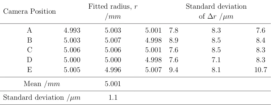
The sphere fit is then further refined by removing 5 % of points with the greatest radial errors, according to Equation (6). With the refined data, the sphere fitting process is repeated to give a final fitted radiusr and the radial errors for the refined points ∆r. The fitted radiusrand the radial errors ∆rcan then be scaled using the fitted radii of the two 5mmspheres. Table 1 shows the fitted radius and standard deviation of the radial errors for all measurements. Table 1 also shows the mean value of all the fitted radii as well as its associated standard deviation.
Camera Position Fitted radius, r /mm
Standard deviation of ∆r /µm
A 4.993 5.003 5.001 7.8 8.3 7.6 B 5.003 5.007 4.998 8.9 8.5 8.4 C 5.006 5.006 5.001 7.6 8.5 8.3 D 5.000 5.000 4.998 7.6 7.1 8.3 E 5.005 4.996 5.007 9.4 8.1 10.7
Mean /mm 5.001
[image:10.612.77.513.92.261.2]Standard deviation /µm 1.1
Table 1. Sphere form and sizing errors
3.2. Sphere spacing error
Using the ball plate described in Section 2.3, the sphere spacing error test was performed as described in Section 2.4. All orientations shown in Figure 5 were measured three times, for all three lengths. As in Section 3.1, the camera was placed in order to produce a magnification of 1:3 such that all three spheres were in focus for the majority of the measurement. Unlike the previous section, the camera was placed at a slightly higher elevation in order to ensure the camera depth of field more evenly covered the ball plate surface.
Again, once all measurements had been taken and reconstructed, all three spheres were fitted using the same process outlined in Section 3.1. The sphere spacing lengths were then calculated according to
Lr,1 =
q
(a1−a2)2+ (b1−b2)2+ (c1−c2)2, (7)
Lr,2 =
q
(a2−a3)2+ (b2−b3)2+ (c2−c3)2, (8)
Lr,3 =
q
(a3−a1)2+ (b3−b1)2+ (c3−c1)2, (9)
whereLr,i is the reconstruction lengthi and [ai, bi, ci] are the coordinates for the centre
of sphere i. For each length, the metric value can then be calculated from
Lm,1 =Lr,1(Lc,3/Lr,3), (10)
Lm,2 =Lr,2(Lc,3/Lr,3), (11)
Lm,3 = 0.5Lr,3((Lc,1/Lr,1) + (Lc,2/Lr,2)) (12)
where Lm,i and and Lc,i are the metric measurement and calibrated value of length i,
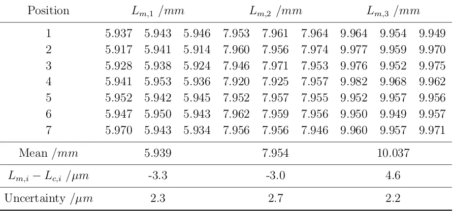
Position Lm,1 /mm Lm,2 /mm Lm,3 /mm
1 5.937 5.943 5.946 7.953 7.961 7.964 9.964 9.954 9.949 2 5.917 5.941 5.914 7.960 7.956 7.974 9.977 9.959 9.970 3 5.928 5.938 5.924 7.946 7.971 7.953 9.976 9.952 9.975 4 5.941 5.953 5.936 7.920 7.925 7.957 9.982 9.968 9.962 5 5.952 5.942 5.945 7.952 7.957 7.955 9.952 9.957 9.956 6 5.947 5.950 5.943 7.962 7.959 7.956 9.950 9.949 9.957 7 5.970 5.943 5.934 7.956 7.956 7.946 9.960 9.957 9.971
Mean /mm 5.939 7.954 10.037
Lm,i−Lc,i /µm -3.3 -3.0 4.6
[image:11.612.74.520.93.301.2]Uncertainty /µm 2.3 2.7 2.2
Table 2. Sphere spacing errors
Table 2 along with the mean of each length, the difference from the calibrated value and the standard deviation on the mean.
Table 2 shows that the system was able to measure lengths between 6 mm and 10 mm, to a standard uncertainty of around 10 µm to 12µm. Based on the maximum permissible error of the sphere spacing calibrations of 0.25µm, the expanded uncertainty on the sphere spacing measurements with a coverage factor of two are 21 µm, 25.2 µm and 20.8 µm for the 6 mm, 8mm and 10mm lengths respectively.
4. Conclusion
characterising the effect of laser speckle for texture projection.
Acknowledgements
The authors would like to thank EPSRC (Grants EP/M008983/1 and EP/L016567/1) for funding this work. We would also like to thank Alexander Jackson-Crisp for helping to manufacture the photogrammetry equipment and Jeremy Straw for calibration using the F25 high-accuracy CMM.
References
[1] Luhmann T, Robson S, Kyle S and Boehm J (eds) 2011Close Range Photogrammetry : Principles, Techniques and Applications (Berlin: Whittles Publishing)
[2] Brown J V-STARS/S Acceptance Test Results (geodedic systems) [3] Chen Z, Liao H and Zhang X 2014Opt. Lasers Eng.57 82–92
[4] Gallo A, Muzzupappa M and Bruno F 2014J. Cult. Herit.15173–182
[5] Percoco G, Lavecchia F and S´anchez Salmer´on A 2015Procedia CIRP 33257–262 [6] Percoco G and S´anchez Salmer´on A 2015Meas. Sci. Technol.26 095203
[7] Koutsoudis A, Ioannakis G, Vidmar B, Arnaoutoglou F and Chamzas C 2015 J. Cult. Herit. 16
664–670
[8] Galantucci L, Pesce M and Lavecchia F 2015 Ann. CIRP - JMST 64507–510 [9] Galantucci L, Pesce M and Lavecchia F 2016 Precis. Eng.43211–219
[10] Eulitz M and Reiss G 2015J. Struct. Biol.191190–196
[11] Fassi I and Shipley D (eds) 2014Micro-Manufacturing Technologies and Their Applications(Berlin: Springer)
[12] Leach R (ed) 2014Fundamental Principles of Engineering Nanometrology (Amsterdam: Elsevier) [13] VDI/VDE 2634 2014Optical 3D – Part 3: Measuring Systems - Multiple View Systems based on
Area Scanning (Berlin – Gesellschaft Mess- und Automatisierungstechnik) [14] Gonz´alez-Jorge H 2011Opt. Eng.50073603
[15] Hastedt H, Ekkel T and Luhmann T 2016Proc. Int. Arch. Photogramm. Remote Sens. Spatial Inf. Sci.XLI-B1851–859
[16] Beraldin J, Mackinnon D and Cournoyer L 2015 Proc. 17th Int. Congress of Metrology 13003
1–21
[17] Lingua A, Marenchino D and Nex F 2009Sensors 93745–3766 [18] Lowe D 2004Int. J. Comput. Vision 6091–110
[19] Pickerd V 2013Technical Notes
[20] Siebert J and Marshall S 2000Sensor Rev.20218–226
[21] Schaffer M, Grosse M and Kowarschik R 2010Appl. Optics 493622–3629
[22] Dainty J C, Ennos A E, Franon M, Goodman J W, McKechnie T S and Parry G 1975 Laser Speckle and Related Phenomena(Berlin: Springer)
[23] Spheric trafalgar ltd http://www.ballbiz.co.uk/uk-spec-prod-reference-tooling-balls.php accessed: 03-11-2016
[24] Spheric Trafalgar Limited 2016 Certification of calibration - 10mm grade 25 tungsten carbide calibration sphere (matt finish) Tech. rep. UKAS
[25] Spheric Trafalgar Limited 2016 Certification of calibration - 5mm grade 25 tungsten carbide calibration sphere (matt finish) Tech. rep. UKAS
[26] Carl Zeiss Industrial Metrology GmbH 2006 F25 - Measuring Nanometres
for Coordinate Measuring Systems (CMS) – Part 8: CMMs with Optical Distance Sensors
(Geneva: International Organization for Standardisation)
[28] ISO 15530 2013 Geometrical Product Specifications (GPS) – Coordinate Measurement Machines (CMM): Technique for Determining Uncertainty of Measurement – Part 3: Use of Calibrated Workpieces or Measurement Standards (Geneva: International Organization for Standardisation)
[29] Agisoft Photoscan: Standard edition, v. 1.2.6 (http://www.agisoft.com/)