System Reliability Evaluation for Imperfect Networks Using Polygon to Chain Reduction

ISSN Online: 2160-8849 ISSN Print: 2160-8830

System Reliability Evaluation for Imperfect

Networks Using Polygon-to-Chain Reduction

Mohamed-Larbi Rebaiaia, Daoud Ait-Kadi

Department of Mechanical Engineering/Interuniversity Research Center on Enterprise Networks, Logistics and Transportation, Laval University, Quebec, Canada

Abstract

The purpose of this paper is to propose a computational technique for eva-luating the reliability of networks subject to stochastic failures. In this com-putation, a mathematical model is provided using a technique which incor-porates the effect of the factoring decomposition theorem using polygon- to-chain and series-parallel reductions. The algorithm proceeds by identifying iteratively one of seven polygons and when it is discovered, the polygon is immediately removed and replaced by a simple chain after having changed the individual values of the reliability of each edge and each node of the polygon. Theoretically, the mathematical development follows the results presented by Satyanarayana & Wood and Theologou & Carlier. The computation process is recursively performed and less constrained in term of execution time and memory space, and generates an exact value of the reliability.

Keywords

Reliability, Networks, Algorithms, Factorization, Polygon-to-Chain Reduction, Decomposition

1. Introduction

Over the last decades, the reliability evaluation of systems and networks has be-come a priority for all manufacturers, particularly in areas when human life is at stake. These areas are especial; aeronautics and telecommunication, nuclear and chemical industries, emissions of greenhouse gases, and many others where high level of service is needed. System reliability is supported very early of the design process. In fact, designers are always trying to develop the best possible product that takes into account its impact on the environment; that must be sustainable and safe, and competitive in term of robustness and evidently that generates earning. Several technical solutions are well-known by designers and engineers;

How to cite this paper: Rebaiaia, M.-L. and Ait-Kadi, D. (2017) System Reliability Eval-uation for Imperfect Networks Using Poly-gon-to-Chain Reduction. American Journal of Operations Research, 7, 201-224. https://doi.org/10.4236/ajor.2017.73014

Received: August 5, 2015 Accepted: August 12, 2015 Published: May 22, 2017 Copyright © 2017 by authors and Scientific Research Publishing Inc. This work is licensed under the Creative Commons Attribution International License (CC BY 4.0).

http://creativecommons.org/licenses/by/4.0/

they are included gradually during the life-cycle of products.

In the literature, dozens of applied methods and techniques have been pro-posed for determining the reliability of networks [1]. Several of them are called enumeration algorithms [2]-[12], summation of disjoint products [5] [8] [13], transformations of star-delta and delta-star structures [14], factoring & Reduc-tion techniques [11] [14]-[22], binary decision diagrams methods [6] [7] [18] [23][24], Bayesian models [25], etc. Simulation and approximating procedures have been used when the problem is tedious or when the exact value of the relia-bility is not necessary required [12][26]. However, most of these solutions are very effective but unfortunately do not allow taking into account the complexity of systems and networks’ architecture. The problem is that, in practice, there is no general and unified mathematical expression that can represent the reliability from which an exact value can be determined, except for some specific architec-ture, such as parallel, series, series-parallel, standby, k-from-n, and others as discussed in the literature (see [27]).

The problem of evaluating the reliability of networks has been verified to be NP-hard [28] and more specifically to be a counting problem or #-P-complete (number P-complete) problem ([28][29] [30]). To avoid such complexity, sev-eral methods and techniques have been proposed, such as factoring and reduc-tions algorithms. Some advised researchers like Wood reported in [31] some advantageous provided by factoring algorithms which require exponential time in the worst case and are at most quadratic in the size of the network because at most |𝐸𝐸| (the cardinal of E) modified copies of the network need ever be main-tained in a stack at any time. He also noted that only a narrow range of reliability measures can be analysed and directed networks are problematic; they can only be handled in a limited way, and this, is considered as a disadvantage.

Moskowitz in 1958 introduced a clever technique based on the well-known Moore & Shannon theorem [15][18][32] [33]. Almost in the same time other researchers proposed a new category of methods which combines the factoring theorem and reduction operations using an efficient procedure that transforms a polygon structure into a simple chain and from which it becomes very easy to determine the reliability [2][15][16][21] [23][30][33][34][35]. Satyanarana and Chang in [35], Satyanarana and Wood in [21] and Wood in [31] for exam-ple, proposed a unified framework based on the factoring theorem to evaluate the reliability of networks whose only nodes are fully reliable, and where any edge is considered as the centerpiece that can be factored, it is called pivot or bridge. A little time later, Theologou and Carlier [22] proposed an original idea which provides a simple mathematical transformation to factoring either on nodes of on edges, but avoids the dependency problem between nodes and edges failures which consider the problem as the well-known common cause problem.

the idea of decomposing the network structure into a well-distinctive compo-nent’s structure and then simplify these components directly into chains of type-1, type-2 until type-7 (see more closely [14][18] to understand the type’s concept) by direct application of the factoring theorem as presented in Equation (3). Type-1 and type-2 are applicable to networks with a source node and a ter-minal node.

To explain the ideas developed in this article about the principle of transfor-mation, we state two theorems that establish some mathematical concepts of transformation. Naturally, it would have been wiser to detail all the transforma-tions of “polygon-to-chain” of any type, but due to the distinctive similarities of the generated mathematical formulas it is quite sufficient to present just type-1 and type-7 reductions, the rest is left as an application exercise to the readers. By against, a summary table reports the results of all these transformations, it is given at the end of this article.

The paper is organized as follows: Section 2 reviews some theoretical back-ground and introduces the factoring theorem. Section 3 presents the operations of reduction polygons-to-chains for imperfect edges and nodes. In Section 4 a practical example is treated for determining the reliability of the proposed net-work, and Section 5 concludes the paper.

2. Backgrounds

2.1. Basic Knowledge

Consider an undirected stochastic network (graph) G=

(

V E, ,

)

where V is a finite set of nodes, E is a finite set of edges, and  represents the probability domain such that each edge/node takes its value from . In other words, it is associated to each edge and/or to each node a real value pi (i: represents the name given to any arc/node). Mathematically speaking, “p qi i ” corresponds to the magnitude given to the probability of functioning/failing of the component i. In this paper, we consider that when a component fails, this does not necessary leads other components to fail, which means that all the components are inde-pendent and the notion of common cause of failure is prohibited. We consider the alphabetic characters s and t for representing the source and the sink nodes of the network. We denote the reliability of the network by R G

( )

K , where K is a specified subset of V with K ≥2. If cardinality of K is equal to 2, the problem is called 2-terminal reliability. A success set, is a minimal set of edges of G such that all the vertices in K are connected. The set is minimal if the deletion of any edge causes the vertices in K to be disconnected and thus the reliability of the network cannot be determined. Two nodes v1 and v2 of the network are

connected if there exists a sequence of nodes and edges of the form

(

) (

)

(

)

1, 1, 1 , ,1 1, 2 , , i, 2 , 2

v v e e e e  e v v (s.t. e_i∈E). Such a sequence is called a path

if the edges are direct. A set of nodes K⊆V is connected if there exists a path

constitutes a polygon. Note that a chain or a path can be interpreted mathemat-ically as a set of elements (nodes and edges). Topologmathemat-ically, a success set is a mi-nimal tree of G covering all vertices in K. Also, we define parallel edges as edges with the same extremities and two adjacent edges are in series if their common nodes are of degree 2 and not in K. We note that replacing a pair of series (pa-rallel) edges by a single edge is called series (pa(pa-rallel) reduction. So, If e is an edge of end-nodes u and v, then

[

G−e

]

(Figure 1: right) is a subgraph of G

obtained by deleting e from G and

[

G e∗

]

represents a subgraph of G obtained

by contracting edge e from G (Figure 1: right). Edge e is considered as a keys-tone edge or the pivot. The edge pivot cannot be chosen arbitrarily [2]. For that, several techniques have been proposed in the literature [3][12]. For some net-works, the K-nodes are represented by solid circles because they are perfect

which means that their reliability value is equal to 1. The rest of the nodes are represented by empty circles and their reliability takes its value in

] [

0,1 ; they are imperfect. When K =E, the problem is treated as: all-terminal reliability,

which mean that all nodes are perfect and the reliability calculus must considers all the relations (paths) between any two nodes of the networks.

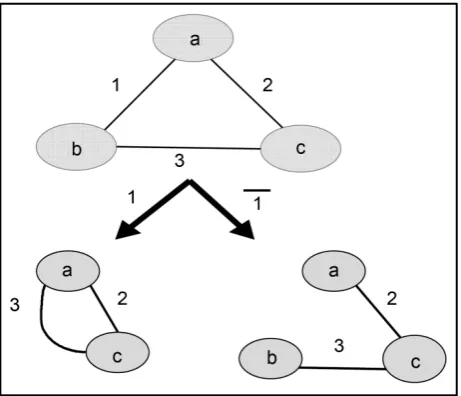
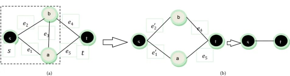
[image:4.595.56.536.599.706.2]

In practice, to reduce the size of the network structure, several reduction rules have been proposed from which series and parallel are the well-known. They are applied only if the network is reducible. In the opposite case, the graph must support any other transformations such as polygon-to-chain reductions (see Figure 1: left).

2.2. The Factoring Principle

The reduction by factorization is based on the factoring theorem of Moore & Shannon theorem [33], which is considered by several authors as the basis for a class of algorithms for computing K-terminal reliability [27] [31]. It consists of decomposing a graph by making assumptions about the state of a component (edge/node) until a simple configuration is obtained. The theorem of total probabilities is then applied to calculate the reliability of this last generated graph. The idea behind this process is to consider an edge e in a graph and to suppose that is still working. This statement is represented mathematically by the function

(

Φ

(

X t

( )

)

=1 |x_e =1

)

where Φ ∗

( )

represents the structure func-tion of the network, and X t

( )

is a vector determining the state of the system.

In other words, it means that the communication through the edge e is provided. In a directed graph, perfect communication between two nodes means that, it is possible to gather them into a single node and the impossibility of communicat-ing through an edge means that the edge must be deleted (see Figure 1 (right part)). Using the theorem of total probabilities (Equation (1)), we can easily compute the reliability of the network.

Note that theorems of Moore & Shannon [33] or the well-known theorem of Bayes [25] and those of Total probabilities are equivalent in our context. We can provide easily mathematical relations between them.

Consider a graph G and a component e∈E selected arbitrary. The theorem

of total probabilities allows for a component e to express the reliability of G as a conditional probability using Equation (1).

( )

(

(

( )

)

)

( )

(

)

(

)

(

)

( )

(

)

(

)

(

)

Pr 1

Pr 1 | 1 Pr 1

Pr 1 | 0 Pr 0

e e

e e

R G X t

X t x x

X t x x

= Φ =

= Φ = − =

+ Φ = = =

(1)

where Pr

(

xe =1

)

is the probability that the component e works and Pr

(

xe =0

)

otherwise, and where Φ

(

X t

( )

)

defines the structure function which represents

the state of the system. In other word, the reliability of the system can be related with the expected mathematical expression which is R G

( )

=E

{

Φ

( )

X

}

(see.

[27]) for explanations.

It follows that if we substitute Pr

(

xe=1

)

by

( )

pe and Pr

(

xe=0

)

by

(

1−pe

)

, yields to the expression of the reliability given by Equation (2).

( )

(

(

( )

)

)

( )

(

)

(

)

( )

(

)

(

)

(

)

Pr 1

Pr 1 | 1

Pr 1 | 0 1

e e

e e

R G X t

X t x p

X t x p

= Φ =

= Φ = =

+ Φ = = −

(2)

This decomposition process continues as many times as it is necessary (recur-sively), until a simple structure is found (if any) and whose reliability is easy to be evaluated. It should be noted that the selection of certain components may sometimes decreases the process of reduction, and therefore the solution is ob-tained more quickly.

From Equation (2), it can be established the validity of the factoring theorem following conditional reliability formula as given by Equation (3):

( )

e

(

)

e

(

)

R G = p R G e∗ +q R G−e (3)

where,

( )

R G : The network reliability.

(

)

R G e∗ : The probability that the system works when the component e

works (edge e is contracted).

(

)

R G−e : The probability that the system works when the component e is

down (edge e is removed). 1

e e

It is easy to say by comparing the Equations (2) and (3) that R G e

(

∗

)

and

(

)

R G−e are none other than Pr

(

Φ

(

X t

( )

)

=1 |xe =1

)

and

( )

(

)

(

)

Pr Φ X t =1 |xe=0 .

The example depicted in Figure 2 illustrates the application of the factoring theorem using component 1 as a pivot. We assume that the node source corres-ponds to the node a and the terminal node is node c. If we apply Equation (3), we obtain the following expression of the reliability:

( )

(

)

(

)

[

]

[ ]

1 2 3 2 3 2

2 1 3 1 2 3

e e

e

R G p R G e q R G e

p p p p p q p

p p p p p p

= ∗ + −

= + − +

= + −

Note that the factoring operation is a special case of pivotal decomposition of a binary system as stated in [16][17].

3. Factorization of Networks with Imperfect Nodes and

Edges

For all the underlying development, we assume the following assumptions: •_{The edges and nodes can fail with a probability} q= −1 p.

•_{The components are s-independent with known probabilities.} •_{All K-nodes are perfectly reliable (}p=1).

3.1. Polygon-to-Chain Reduction

The objective of substituting a polygon by a chain is an action used to reduce the calculation of the reliability when traditional algorithms are not able to provide a finite solution or when the graph is irreducible. For that, Satyanarayana and Wood have identified seven types of polygons and presented their equivalent mathematical expressions [21] [31]. A table covering these polygons and their equivalences is published in [21] just for networks with perfect nodes.

[image:6.595.258.489.517.715.2]

The reduction polygon-to chain in the case of imperfect graphs is further

complicated because the transformation must to take into account the state-ments of nodes and edges at the same time. Several authors have mentioned this difficulty [2] [3] [23] [30] [36]. Theologou and Carlier [22] first, have argued that when pivoting on a node, the transformation problem becomes more com-plex and consequently the graph augments in its size.

In this paper we propose an algorithm which combines the reduction poly-gon-to-chain using the works of Theologou and Carlier [22], those of Satyana-rayana and Wood [21], Simard [14] and Rebaiaia and Ait-Kadi [27], in the sense that a combination of Satyanarayana and Wood [21] and of Theologou and Car-lier [22] are provided. We find the work of Theologou and Carlier [22] very in-teresting because their technique avoids the problem of dependency between the network components’ failures. These assumptions are summarized as follows:

Consider the link e=

( )

u v, , where u and v are two imperfect nodes. We suppose that any link l works with a probability pl when e, u and v work with their respective probabilities p ii

(

=e u v, ,

)

. Then pl can be written using the following equation:

l e u v

p =p p p (4)

We note that the pivoting on the link l by applying the factoring theorem produces the contraction of the edge e and the merging of edges u and v, and this operation creates a new perfect node. By cons, if the link fails, the cause of the failure cannot be known a priori, because it could be that one of the three components of the link has failed, and the relative conditional probabilities are given by Equations (5) and (6). Anyway, this link will be lost and therefore it will be deleted.

After this operation of pivoting, the reliabilities of nodes v and u will be iden-tified by the following new expressions:

(

)

(

)

Pr works | or or are down v u u e

v v u u e

v

v

p q p q

p v v e u

q p q p p q

+

′ = =

+ + (5)

(

)

(

)

Pr works | or or are down u v v e

u u v v e

u

u

p q p q

p u u e v

q p q p p q

+

′ = =

+ + (6)

We can remark that Equations (5) and (6) show clearly that u and v are inti-mately connected. Thus, to avoid such dependency and for respecting the initial assumptions, Theologou and Carlier in [22] proposed a new expression representing the probability of u and v. The idea is as follows:

Suppose that all the K-nodes of the graph are full connected between them-selves, that is, if this is not the case, the reliability of the original network is equal to,

( )

K v

( )

v K K

R G p R G

∈

′

=

∏

₍₇₎

where GK and G′K contain K-imperfect nodes. They are the initial graph and its reduced one. Then there exists at least two K-nodes and it is always possible to find an edge in the graph with one of its end-node be perfect.

and because pv≠1, the relation (8) is then obtained.

(

v e

)

v

v v e

p q p

q p q

′ =

+ (8)

Note that in the present state, the failure node v depends only on the link e

and therefore e, u and v are now independent.

As the node v remains in the graph or the link l is down, then the other links that have one of their extremities as node v can now be factored and the failure of node v depends only on the failure of these edges. Therefore, we can now de-termine the general formulation for representing the reliability of the imperfect node v at any stage of the factoring process when edges

(

e e1, 2,,er

)

incident to v are factored. Consequently we obtain the reliability p′′v after applying the factoring theorem as given by Equation (9).

(

)

(

)

(

1

)

1 1

Pr fonctionne | ou en panne ou en panne

j

j

v r

r

v j e

r

v v j e

p v v e v e

p q

q p q

=

=

′′ = ∧ ∧

= +

∏

∏



(9)

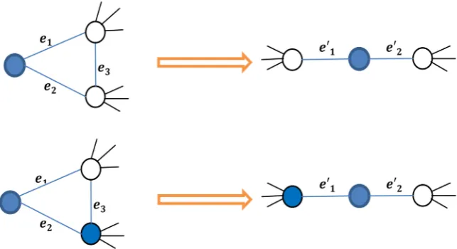
In the sequel, we present the first transformation of polygon-to-chain using the factoring process. Here the polygon of type-1 is a triangle and a chain is two successive edges that can be reduced to one edge with its end-points (see Figure 3). As you can see in Figure 3, the triangle structure must contain at least one perfect node. If it contains two perfect nodes, it is named polygon of type-2.

3.1.1. Polygon-to-Chain Reduction of Type-1 (Type-2) for a K-Terminal Reliability

[image:8.595.211.533.538.713.2]

Consider a graph containing a polygon of type-1 or of type-2 as presented in Figure 3 (left, up/down) and let ps, pa et pb be the individual reliabilities at nodes s, a and b. Remember that the node s is the initial node and it is perfect, while a and b are imperfect. Note that type-1 polygon is a partial-graph and type-2 is a 2-terminal network [36]. Both of them are also known as trian-gle-network. Note also that this paper considers that nodes and edge both of

them maybe subject to random failures. We can now state the following theorem:

Theorem 1.

Suppose G be a graph containing a polygon of type-1 as shown if Figure 3 (up/left). Let G′ denotes the reduced graph generated after transforming G by

replacing edges e1 and e2 by edges e1′ and e2′ of reliabilities p1′ and p2′

(e3 is simply deleted). Suppose also that the reliability at node a and b are respec-tively pa′ and p2′ (Figure 3 (up/right)), and let Ω be the multiplier factor

also called the transformation factor. Then the reliability of the network is:

( )

( )

R G = ΩR G′ (10)

where Ω =

(

δ

+A

)(

δ

+B

)

δ

, p1′ =

δ δ

(

+AC

)

, p2′ =

δ δ

(

+BD

)

,

(

) (

)

a

p′ =

δ

+AC

δ

+A , pb′ =

(

δ

+BD

) (

δ

+B

)

such that:

[

]

[

]

[

]

(

)

(

)

1 2 1 3 2 3 1 2 3 2 1 3 1 3 1 2 3 2 3

1 3 1 3 2 3

2 3

2 1

1 a b

b a a a

a b b b

a

a a

b

b b

p p p p p p p p p p p

A p p p p p p p p p

B p p p p p p p p p

p q q C

q p q q

p q q D

q p q q

δ

 = + + −



= − − +



 = − − +

 

=

 ₊

 

= 

+ 

(11)

Proof:

Assume that we are in the presence of a graph G which contains at least one polygon of type-1. Then the reduced subgraphs

(

G e∗ 1

)

and

(

G−e1

)

are

ob-tained by applying the factoring theorem (Equation (3)) using the link

(

s e a, ,1

)

as a pivot and are used to determine the reliability expression of the graph G in Equation (12).

( )

1 a

(

1

) (

1 1 a

) (

1

)

R G = p p R G e∗ + −p p R G−e (12)

Assume now that a is a node pivot. After applying Equation (8) to the node a

the reliability of the node a in the subgraph

(

G−e1

)

is represented by Equation

(13):

(

a 1 1

)

a

a

a p q p

q p q

′ =

+ (13)

Then, when pivoting on the link

(

s e b, 2,

)

, the factoring on the reduced

sub-graphs G e∗ 1 and G−e1, generates the new reduced subgraphs

(

)

(

G e∗ 1 ∗e2

)

,

(

(

G e∗ 1

)

−e2

)

,

(

(

G−e1

)

∗e2

)

and

(

(

G−e1

)

−e2

)

. The last

sub-graph is systematically eliminated because at this level of development, the link between node s and node a, and node s and node b are broken. The reliability expression of the graph G at this step becomes:

( )

(

(

)

)

(

) (

(

)

)

(

)

(

(

)

)

1 2 1 2 2 1 2 1 2 1 2

1

1 *

a b b

a b

R G p p p p R G e e p p R G e e

p p p p R G e e



= _ ∗ ∗ + − ∗ − _

 

+ − _ − _ (14)

sub-graph

(

G e∗ 1

)

−e2 is given by Equation (15).

(

2 2

)

b b

b b

p q p

q p q

′ =

+ (15)

By decomposing successively on the link

(

s e b, ,3

)

in the reduced graph

(

G e∗ 1

)

−e2 and on the link

(

s e a, ,3

)

in the reduced graph

(

G−e1

)

∗e2, then,

the new expression of the system reliability is:

( )

(

(

)

)

(

)

(

(

(

)

)

)

(

)

(

(

(

)

)

)

(

(

)

)

(

)

(

(

)

)

(

) (

(

)

)

1 2 1 2 2 3 1 2 3

3 1 2 3 2 1 2

1 2 3 1 2 3 3 1 2 3

1

1

1 1

a b b b

b b

a b a a

R G p p p p R G e e p p p p R G e e e

p p R G e e e p p R G e e

p p p p p p R G e e e p p R G e e e

  ′

= _ ∗ ∗ + − _ ∗ − ∗

 

 

′

+ − ∗ − − _ − ∗ _

  ′ ′ 

+ − _{ } − ∗ ∗ + − − ∗ − _

(16)

In the sub-graph

(

(

G−e1

)

∗e2

)

−e3 generated in Equation (16), the new

value of the reliability of the node a is equal to:

(

1 31 3

)

a a

a a

p q q p

q p q q

′′ =

+ (17)

Likewise for the graph

(

(

G e∗ 1

)

−e2

)

−e3, the reliability of the node b is:

(

2 32 3

)

b b

b b

p q q p

q p q q

′′ =

+ (18)

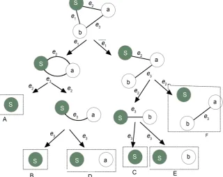
[image:10.595.215.536.446.701.2]

Note that several states can induce the same graph. To get an idea on the con-cept of equivalence in this direction (see Figure 4 (terms A, B and C)) to recover the equivalent substructures in terms of reliability. We can now establish the following equalities:

Figure 4. Graph of type-1 and its series of successive transformations par application of

(

)

(

1 2

)

(

(

(

1

)

2

)

3

)

(

(

(

1

)

2

)

3

)

R G e∗ ∗e =R G−e ∗e ∗e =R G e∗ −e ∗e (19)

By grouping (A, B, C and D, E) and eliminating the configuration F, the sys-tem reliability becomes:

( )

[

]

(

(

)

)

[

]

(

(

(

)

)

)

[

]

(

(

(

)

)

)

1 2 1 3 2 3 1 2 3 1 2 1 2 3 2 3 1 2 3 2 1 3 1 3 1 2 3

2

1

1 a b

a b b b

b a a a

R G p p p p p p p p p p p R G e e

p p p p p p p p p R G e e e

p p p p p p p p p R G e e e

= + + − ∗ ∗

+ − − + ∗ − −

+ − − + − ∗ −

(20)

Assume G′ is obtained from G after the reduction process. Then by

fac-toring on the link

(

s e a, ,1′ ′

)

, the reliability of the system G′ is:

( )

1 a

(

1

) (

1 1 a

) (

1

)

R G′ = p p R G′ ′ ′ ′∗e + −p p′ ′ R G′−e′ (21)

The reliability of the node a′ in the graph

(

G′−e1′

)

is equal to:

( ) (

1 1

)

a a

a a

p q p

q p q

′ ′ ′ ′ ′ ′ ′ ′ =

′ + ′ ′ (22)

A similar way is applied to the node b′ giving the following reliability

ex-pression as shown in (23):

( ) (

2 2

)

b b

b b

p q p

q p q

′ ′ ′ ′ ′ ′ ′ ′ =

′ + ′ ′ (23)

Finally, the reliability expression of G′ is given by Equation (24).

( )

1 a 2 b

(

(

1

)

* 2

)

(

1 2 b

) (

(

1

)

2

)

R G′ = p p′ ′′p p R′ ′ G′ ′∗e e′ + −p p′ ′ R G′ ′∗e −e′  (24)

Because the graphs G and G′ are equivalent respecting to relation (10), we

get the following equalities’:

(

)

(

1 2

)

(

(

1

)

2

)

R G e∗ ∗e =R G′ ′∗e ∗e′ (25)

(

)

(

)

(

1 2 3

)

(

(

1

)

2

)

R G e∗ −e −e =R G′ ′∗e −e′ (26)

Now, we remark that Equation (26) is valid if and only if the relations (27), (28) and (29) are respected.

( )

a a

p′′= p′ ′ (27)

(

)

(

)

(

1 2 3

)

(

(

1

)

2

)

R G−e ∗e −e =R G′−e′ ∗e′ (28)

( )

b b

p′′= p′ ′ (29)

Due to Equations (10), (25) and (26), we can determine the following system:

[

]

[

]

[

]

(

)

[

]

(

)

(

) (

)

(

) (

)

1 2 1 3 2 3 1 2 3 1 2 1 3 3 2 3 2 1 3 1 3

1 3 1 3 2 3 2 1 2 1 2 1 2 1 3 1 2 2 2 Ω

1 Ω 1

1 Ω 1

a a b

a b b b

b a a a

a a

a a a a

b b b b a b b b b a b

p p p p p p p p p p p p p p p

p p p p p p p p p p p p p p p

p p p p p p p p p p p p p

p q q p q

q p q q q p q

p q q p q

q p q q q p q

By solving the system in (30), the values of Ω,p p1′ ′ ′, 2,pa and p′b are up-dated according to:

(

)(

)

(

)

(

)

(

)

(

)

(

)

(

)

1

2

a

b

A B

p

AC

p

BD

AC p

A

BD p

B

δ δ

δ δ δ

δ δ

δ δ δ

δ

′

′



+ +

Ω =    ′ =

 +

  ′ = 

+ 

 ₊

 ′ = + 



+  ′ =

 ₊



(31)

where δ, A, B, C and D are identified by the following relations:

[

]

[

]

[

]

(

)

(

)

1 2 1 3 2 3 1 2 3 2 1 3 1 3 1 2 3 2 3

1 3 1 3 2 3

2 3

2 1

1 a b

b a a a

a b b b

a

a a

b

b b

p p p p p p p p p p p

A p p p p p p p p p

B p p p p p p p p p

p q q C

q p q q

p q q D

q p q q

δ

 = + + −



= − − +



 = − − +

 

=

 ₊

 

= 

+ 

(32)

Finally, we note that it is possible to derive a simplified topology from another more complex by applying a series of reductions using the factoring theorem while keeping unchanged the value of the reliability of a network. The problem that may arise is how to automating the recognition of such topologies whose calculations can be deduced easily. The idea is very beneficial provided to design algorithms that easily skip such a critical stage of the calculation process, or at least to determine the necessary means to seek equivalencies between structures. To deal with such problems, two interesting productions challenge us; they have been reported independently in [19] and [22].

Now, we skip the determination of the mathematical relations between the original graph and its reduced graph for the cases of type-2 to type-6, the rea-soning scheme is particularly the same as of type-7. At the end of the paper a ta-ble is provided to resume the reductions relative to polygon-to-chain of type-1 to type-7.

Note that type-2 polygon-to-chain reduction generates the same mathematical relations given in systems (31) and (32). The verification is left to the reader.

3.1.2. Polygon-to-Chain Reduction of Type-7

case to represent the subgraphs, events-states and all the reductions, they are represented in Table 1. Before that, we present the following theorem which states the principle of polygon-to-chain of type-7 reduction. It provides all the equivalence expressions. To prove the theorem, we proceed by factoring the edges and nodes of the graph G, and then, on the reduced graph G′. Finally we

establish the equivalences by correspondence using Equation (10).

Theorem 2.

Let G be a graph containing a polygon of type-7 as presented in Figure 5, and

G′ be the reduced graph generated after transforming G by replacing edges

1, 2, 3, 4, 5, 6

e e e e e e of reliabilities p p1, 2,p p3, 4,p p5, 6 by edges e1′ and e2′ of

[image:13.595.260.490.269.417.2]

reliabilities p′1 and p′2, and nodes a and b of reliabilities pa and pb by the updated reliabilities pa′ and pb′ (See Figure 6). If Ω is the multiplier factor,

Figure 5. Polygon-to-chain reduction of type-7.

Figure 6. The graphs induced using the reduction polygon-

[image:13.595.259.487.448.706.2]

[image:14.595.209.531.89.387.2]

Table 1. Reduced graphs, state vectors and their corresponding probabilities.

GA States Probabilities

B1 F F F F F F F Fa 1 2 3 a 4 5 6

( )( )

( )

2 3 5 6 1 4

2 3 5 6 1 4 1 4

1 1

1

b a a

b a a a

p p p p p p p p p

p p p p p p p p p p p p

α= − −

= − − +

C1 F F F F F F F Fa 1 b 3 4 5 b 6

( )( )

( )

1 2 4 5 3 6

1 2 4 5 3 6 3 6

1 1

1

a b b

a b b b

p p p p p p p p p

p p p p p p p p p p p p

δ= − −

= − − +

D1

1 2 3 4 5 6

a b

F F F F F F F F;

1 2 3 4 5 6

a b

F F F F F F F F;

1 2 3 4 5 6

a b

F F F F F F F F;

1 3 4 5 6

a b

F F F F F F F;

1 2 3 4 5 6

a b

F F F F F F F F;

1 2 3 4 5 6

a b

F F F F F F F F;

1 2 3 4 5 6

a b

F F F F F F F F

3 4 2 5 2 4

1 2 3 4 5 6

3 4 2 5 2 4

1 5 1 6 3 5 2 6

1 5 1 6 3 5 2 6

a b

q q q q q q

p p p p p p p p

p p p p p p

q q q q q q q q

p p p p p p p p

β= _ + + 

+ + + + _



E1

1 2 3 4 5 6

a b

F F F F F F F F;

1 2 3 4 5 6

a b

F F F F F F F F ;

1 2 3 4 5 6

a b

F F F F F F F F ;

1 2 3 4 5 6

a b

F F F F F F F F ;

1 2 3 4 5 6

a b

F F F F F F F F ;

1 2 3 4 5 6

a b

F F F F F F F F

3 5 6

1 2 4

1 2 3 4 5 6

1 2 3 4 5 6

1

a b

q q q

q q q

p p p p p p p p

p p p p p p

γ= _ + _

 + + + + + 

then the reliability of the original graph G is determined using the following re-lations:

(

)(

)(

)

1 3 2 2 a b p C p p D C p D p

γ α γ β δ γ γ γ γ α γ γ β γ γ δ γ α γ α γ δ γ δ  + + + Ω =    ′ =  _{+ ⋅}   ′ =  ₊    ′ =  + ⋅  + ⋅  ′ =  ₊  + ⋅  ′ =  ₊  (33)

and such that:

[

]

1 2 3 5 6 1 4 1 4

3 4 2 5 2 4 1 5 1 6 3 5 2 6 1 2 3 4 5 6

3 4 2 5 2 4 1 5 1 6 3 5 2 6 3 5 6

1 2 4 1 2 3 4 5 6

1 2 3 4 5 6 1 2 4 5 3 6 3

1

1

1

b a a a

a b

a b

a b b

p p p p p p p p p p p p p

q q q q q q q q q q q q q q

p p p p p p p p

p p p p p p p p p p p p p p

q q q

q q q

p p p p p p p p

p p p p p p

p p p p p p p p p p p

α β γ δ = − − +   = _ + + + + + + _     = _ + + + + + + _  

=

[

− − + ₆p_b

]

Proof:

Consider a graph containing a polygon of type-7 as depicted in Figure 5 (G). By pivoting successively on edges e e e e e1, 2, 3, 4, 5 and e6, we obtain the

sub-graphs reported in Figure 6; they are five. The corresponding events and proba-bilities are presented in Table 1.

Because the decomposition process uses the links e1 and e4 as pivots in the

reduced graphs B1 (Table 1) and uses the links e3 and e6 as pivots in the

graph C1 (Table 1), then the new reliabilities of the nodes a and bare given by the following equations:

1 4 1 4

a a

a

a

p q q p

q p q q

′′ =

+ (35)

3 6 3 6

b b

b

b

p q q p

q p q q

′′ =

+ (36)

Continuing the application of the factoring theorem on the reduced graph G′

of G (polygon of type-7) and let e e1′ ′, 2 and e3′ the edges of G′.Table 2 gives

the subgraphs generated by the decomposition, and their relative state vectors and probabilities.

The following graph in Figure 7 shows how the state’s formulas and their probabilities are determined. The results of the transformations are presented in Table 2.

Note that, for the graphs B’ and C’, the conditional probabilities for node a

and the link e1′ (graph B’), and for node b and the link e3′ (graph C’) are given

by the following equations:

Table 2. Non-defaulting states and the probabilities induced by the decomposition

process of the graph GK′′.

Graph State Probability

B’ F F F F Fa 1 2 3 b α ′= −

(

1 p p1′ ′a

)

p p p′ ′ ′2 3 b C’ F F F F Fa 1 2 3 b δ ′= −

(

1 p p3′ ′b

)

p p p1′ ′ ′2 a D’ F F F F Fa 1 2 3 b β ′=p q p p p1′ ′ ′ ′ ′2 3 a b E’ F F F F Fa 1 2 3 b γ ′=p1′p2′p p p3′ ′ ′a b

( ) (

1 1

)

a a a a a p q p p

q p q

′ ′ ′

′′ ′ =

′ ′ ′

=

+ (37)

( ) (

3 3

)

b

b b

b b

p q

p p

q p q

′ ′ ′

′′= ′ =

′+ ′ ′ (38)

We can use now the relation R G

( )

= ΩR G′

( )

(Equation (10)) to identify

from Equations (38), (39), (40) and system (41) the coefficients

α β δ

, , and

γ

as presented in the theorem statement.

Using Equation (10), we obtain the following relations:

(

)

(

)

(

)

(

)

(

)

(

)

(

)

(

)

, , , ,

, , , ,

B C D E

B C D E

B K C K D K E K

B K C K D K E K

R G R G R G R G

R G R G R G R G

α δ β γ

α ′ _′ β ′ _′ δ ′ _′ γ ′ _′

⋅ + ⋅ + ⋅ + ⋅

 ′ ′ ′ ′ ′ 

= Ω_ + + + _ (39)

Using Equations (35), (37) and (38) we can identify the following relations:

(

)

1 4

1 4 1

1 a a a a a a

p q q p q

q p q q q p q

′ ′ =

′ ′ ′

+ + (40)

(

)

1 4

1 4 1

1 a a a a a a

p q q p q

q p q q q p q

′ ′ =

′ ′ ′

+ + (41)

We equate now the terms of the Equation (39), it follows the following rela-tions:

[

]

3 5 6 1 2 4

1 2 3 4 5 6

1 2 3 4 5 6

3 4 2 5 2 4 1 5 1 6 3 5 2 6 1 2 3 4 5 6

3 4 2 5 2 4 1 5

1 2 3

1 1 6 3 5 2 6 1 2 4 5 3 6

2 3 3 6 1 Ω Ω 1 a b a b

a b b

a b

b

a b

q q q

q q q

p p p p p p p p p p p p

p p p p p p

q q q q q q q q q q q q q q

p p p p p p p p p q p p p

p p p p p p p p p p p

p

p p p

p p p p p p p p p p p p

  ′ ′ ′ ′ + + + + + + =       _{′ ′ ′ ′ ′} + + + + + + =     − − + ′ =

(

)

[

]

(

)

(

) (

)

(

) (

)

1 2 3 5 6 1 4 1 4 1 4

1 4 3

3 1 2

6 3 6

1 2 3 1

1 3

3

Ω 1

1 Ω 1

b a

a b

a

a a

b a a a

a

a a

b b

b

b b b

p

p

p p p p

p p p p p p p p p p p p p p p p p

p q q p q

q p q q q p q

p q q p q

q p q q q p q

′ ′ ′ ′ − ′ ′ ′ ′ − − + = − ′ ′ = ′ ′ ′ +        + ′ ′ = ′ ′ ′ +  ′   ′     +     (42)

By solving the system (42), we identify the expressions of

α β δ

, , and

γ

stated in the Theorem 2 and from which it can be deduced the values of proba-bilities of the reduced graph.

[

]

1 2 3 5 6 1 4 1 4

3 4 2 5 2 4 1 5 1 6 3 5 2 6 1 2 3 4 5 6

3 4 2 5 2 4 1 5 1 6 3 5 2 6 3 5 6

1 2 4 1 2 3 4 5 6

1 2 3 4 5 6 1 2 4 5 3 6 3

1

1

1

b a a a

a b

a b

a b b

p p p p p p p p p p p p p

q q q q q q q q q q q q q q

p p p p p p p p

p p p p p p p p p p p p p p

q q q

q q q

p p p p p p p p

p p p p p p

p p p p p p p p p p p

α β γ δ = − − +   = _ + + + + + + _     = _ + + + + + + _  

=

[

− − + ₆p_b

]

         

(

)(

)(

)

2

γ α γ β δ γ γ

+ + +

Ω = _; p₁

C

γ γ α

′ =

+ ⋅ ; p2

γ γ β

′ =

3 p

D

γ

γ δ

′ =

+ ⋅ ; a

C

p γ α

γ α

+ ⋅ ′ =

+ ; b

D

p γ δ

γ δ

+ ⋅ ′ =

+

At this step, we state that all the mathematical relations are clearly identified, and the values of the probabilities of the reduced graph components (nodes and edges) can be calculated at each step of the reduction process until the final re-duced graph which corresponds to a chain.

Thus, the following algorithm presents the different steps to reach the solution.

3.2. Algorithm Description

Begin

Input data: structure of the graph and the probability of nodes and edges

(

,

)

G= V E : Graph must be composed by one connected component (V:

nodes; E: Edges)

(

)

, ,

i j i j

P = E E : Associated matrix constructed from the edges of the graph

, 2

K⊆V K ≥

1

M =

While there is a simple reduction of the following types: Call procedures:

-Series reductions: Pi =Pj×Pk ; remove the link

(

E Ei, j

)

and

updating the probability vector and the matrix associated with the graph. -Parallel reduction R G

( )

= ΩR G′

( )

: Pi= − −1

(

1 Pj

)

× −

(

1 Pk

)

; re-

move one of the links and update the vector of probabilities and the matrix asso-ciated with the graph.

-Reduction of degree 2. Let M =M× Ω for each reduction. end_while.

Start by exploring the complex substructure (polygons). Let s the initial node.

Determine the ascending nodes of the first, the second level and the lower le-vels, according to the polygon type)

While a polygon exists

If a polygon of type T exists, apply the corresponding reduction of this type of subgraph. Note: One always begins with seeking that of type 1, type 2, etc.

- Store in a stack the links to be removed.

- Remove the corresponding links in the graph associated matrix.

- Rebuilt the new chains from the links stored by forging the links in the matrix of associated graph

- Update the vector of probabilities with the new values for each type T.

- Update the vector of probabilities.

- Update the associated matrix of the graph.

Construct the graph from the resulting matrix.

if the obtained matrix is a simple one

Calculating the reliability as the product of probability links else

Print “Matrix is no longer decomposable”

Apply any other algorithm that calculates the reliability (SDP BDD…) end_if

Display the reliability value of the graph G

end_of_the algorithm.

4. Application

Suppose that the nodes and edges all are imperfect except the initial and the terminal nodes (s, t). We consider that their associated probability values are equal to 0.9. The probabilities value of nodes s and t are equal to 1. Using the following network

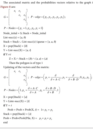
[image:18.595.205.533.298.754.2]

The associated matrix and the probabilities vectors relative to the graph in Figure 8 are:

1 2

3 5

4

e e

e e

G

e

 

 

 

=

 

 

 

; P−edge=

(

p p p p p1, 2, 3, 4, 5

)

;

(

s 1, a, b, t 1

)

P−Nodes= p = p p p =

Node_inital = S; Stack = Node_inital List-succ(s) = (a, b)

Stack = Stack ∪ _{List-succ(s) (queue = {s, a, b}} X = pop(Stack) = {b}

Y = List-succ(X) = {a, t} if Y ≠_t

Z = X ∩ _{Stack = (b)} ∩ _{(s, a) = (a)} Then the polygon is of type 1 Updating of the vectors and the matrix:

1 2

5

4

e e

e G

e

 

 

 

=

 

 

 

; P edge p1 ,p2 , 0,p p4, 5

A C B D

δ

δ

δ

δ

 

− =_ = = _

+ ⋅ + ⋅

 ;

1, a , b ,1

A C B D

P Nodes p p

A B

δ

δ

δ

δ

+ ⋅ + ⋅

 

− =_ = = _

+ +

 

X = pop(Stack) = {a} Y = Liste-succ(X) = {t} if Y = t

Prob = Prob × Prob(X, t) = 1×p5= p5

Stack = pop(Stack) = {s}

[image:19.595.60.537.64.189.2]

(a) (b)

Figure 8. A simple testing graph: (a) the original graph, (center) parallel-series reduction, (b) the reduced graph (chain).

Updating of the vectors and the matrix:

( )

1 ,

e′ = s a

2 1

4

e e

G

e

′

 

 

 

=

 

 

 

; 1 , 2 , 0, 4, 0

.

P edge p Prob p p

B D

δ

δ

 

− =_ = = _

+

 ;

Prob = 1

Liste-succ(s) = {b}

Stack = Stack ∪ _{Liste-succ(S) ( then Stack = (s, b))} X = pop(Pile) = {b}

Y = Liste-succ(X) ={t} if Y = t

Prob = Prob × Prob(X, t) = 1×p4= p4

Stack = pop(Stack) = {s}

Prob = Prob × Prob(Pile, X) = p4×p2×pb Updating of the vectors and the matrix:

( )

2 ,

e′ = s t

1 2

e e

G

′ ′

 

 

 

 

 

 



; P−edge=

(

p1=Prob p, 2=Prob, 0, 0, 0

)

;

(

) (

)

(

1 1 1 1 1 1 , 0, 0, 0, 0

)

P−edge= p′′= − −q × −q end_if

end_Algorithm

Calculus:

function imperfect() p1 = .9

p2 = .9 p3 =.9 pa = .9 pb = .9

A = p2*pb*(1-p1*pa-p3*pa+p1*p3*pa) B = p1*pa*(1-p2*pb-p3*pb+p2*p3*pb)

C=(pa*(1-p1)*(1-p3))/((1-pa) +pa*(1-p1)*(1-p3)) D=(pb*(1-p2)*(1-p3))/((1-pb) +pb*(1-p2)*(1-p3)) omega = (delta + A)*( delta + B)/ delta

p1p = delta /( delta + A*C) p2p = delta /( delta + B*D) pap = (delta + A*C)/( delta + A) pbp = (delta + B*D)/( delta + B) x = 1-(1-p1p*pbp*.9)*(1-p2p*pap*.9) y = x*.81*omega

end

A = B = 0.08829; eta = 0.78732; C = D = 0.0825688073394495; p1p = p2p = 0.990825688073394; pap = pbp = 0.907493061979649; omega =

0.9738008333333333.

As the graph turned into two parallel chains, the reliability of the network is computed as follows:

R = 1 – (1 – p2p*pbp * p4)*(1 – p1p*pap * p4) = 0.963614702184995

R(G) = R * omega * Ps * Pt = 0.963614702184995 * 0.9738008333333333 * 0.9 * 0.9 * = 0.760078728.

5. Conclusion

This paper presents a computational technique determining the reliability of networks. In such networks, it is considered that edges and nodes can fail ran-domly and the failure events are supposed to be s-independent or not. The used techniques combine some algorithms based on the factoring theorem and se-ries-parallel reductions. The algorithm tries first to identify seven types of struc-tures if possible and when one of them is found, such structure is removed and replaced by a more simple chain. Logically, all the remained components’ values are substituted by new values determined by the derived mathematical expres-sions. The correctness of the algorithm is not hard to show and it can be ob-served that at most 2E −V can ever pass through T (T is a stack structure)

before T becomes empty (Satyanarayana and Wood (1985)) and the algorithm still of linear complexity. These techniques are very easy to be integrated to a large software reliability system that can also determine solutions for optimizing the reliability, the availability and the maintainability of critical systems’ design. Future extensions of this work consist of determining some efficient procedures and heuristics to select edges and nodes that can be primary used as pivot for generating the most possible fast solution.

References

[1] Institute of Electrical and Electronics Engineers (1990) IEEE Standard Computer Dictionary: A Compilation of IEEE Standard Computer Glossaries. IEEE Std 610, 1-217.

[3] Dotson, W.P. and Gobien, J. (1979) A New Analysis Technique for Probabilistic Graphs. IEEE Transactions Circuits and Systems, 26, 855-865.

https://doi.org/10.1109/TCS.1979.1084573

[4] Fratta, L. and Montanari, U.G. (1973) A Boolean Algebra Method for Computing the Terminal Reliability in a Communication Network. IEEE Transactions on Cir-cuit Theory, 20, 203-211. https://doi.org/10.1109/TCT.1973.1083657

[5] Heidtmann, K.D. (1989) Smaller Sums of Disjoint Products by Subproduct Inver-sion. IEEE Transactions on Reliability, 38, 305-311.

https://doi.org/10.1109/24.44172

[6] Kuo, S.Y., Yeh, F.M. and Lin, H.Y. (2007) Efficient and Exact Reliability Evaluation for Networks with Imperfect Vertices. IEEE Transactions on Reliability, 56, 288- 298. https://doi.org/10.1109/TR.2007.896770

[7] Lin, H.Y., Kuo, S.Y. and Yeh, F.M. (2003) Minimal Cutset Enumeration and Net-work Reliability Evaluation by Recursive Merge and BDD. Proceedings of the 8th IEEE International Symposium on Computers and Communication,2, 1530-1346. [8] Liu, H.H., Yang, W.T. and Liu, C.C. (1993) An Improved Minimizing Algorithm for

the Summation of Disjoint Products by Shannon’s Expansion. Microelectronic Re-liability, 33, 599-613.

[9] Misra, K.B. (1970) An Algorithm for the Reliability Evaluation of Redundant Net-works. Transactions on Reliability, R-9, 146-151.

https://doi.org/10.1109/TR.1970.5216434

[10] Tarjan, R.E. (1972) Depth First Search and Linear Graph Algorithms. SIAM Journal of Computing, 1, 146-160. https://doi.org/10.1137/0201010

[11] Yan, L. and Taha, H.A. (1994) A Recursive Approach for Enumerating Minimal Cutsets in a Network. IEEE Transaction on Reliability, 43, 383-388.

https://doi.org/10.1109/24.326430

[12] Yoo, Y.B. and Deo, N. (1988) A Comparison of Algorithms for Terminal-Pair Re-liability. IEEE Transactions on Reliability, 37, 210-215.

https://doi.org/10.1109/24.3743

[13] Locks, M.O. and Wilson, J.M. (1992) Note on Disjoint Products Algorithms. IEEE Transactions on Reliability, 41, 81-84. https://doi.org/10.1109/24.126676

[14] Simard, C. (1996) Contribution au problèmed’évaluation de la fiabilité des réseaux. Master Thesis, Laval University, Quebec, Canada, TJ-7.5-UL-1996.

[15] Moskowitz, F. (1958) The Analysis of Redundancy Networks. Transactions of the American Institute of Electrical Engineers, Part I: Communication and Electronics, 77, 627-632.

[16] Page, L.B. and Perry, J.E. (1988) A Practical Implementation of the Factoring Theo-rem for Network Reliability. IEEE Transactions on Reliability, 37, 259-267.

https://doi.org/10.1109/24.3752

[17] Page, L.B. and Perry, J.E. (1989) Reliability of Directed Network Using the Factor-ing Theorem. IEEE Transactions on Reliability, 38, 556-562.

https://doi.org/10.1109/24.46479

[18] Rebaiaia M.L. (2011) A Contribution to the Evaluation and Optimization of Net-works Reliability. PhD Thesis, Laval University, Canada.

[19] Resende, M.G.C. (1986) A Program for Reliability Evaluation of Undirected Net-works via Polygon-to-Chain Reductions. IEEE Transaction on Reliability, 35, 24-29.

https://doi.org/10.1109/TR.1986.4335334

Theorems. Networks, 13, 107-120. https://doi.org/10.1002/net.3230130107

[21] Satyanarayana, A. and Wood, R.K. (1985) A Linear-Time Algorithm for Computing K-Terminal Reliability in Series-Parallel Networks. SIAM Journal on Computing, 14, 818-832. https://doi.org/10.1137/0214057

[22] Theologou, R. and Carlier, J.G. (1991) Factoring & Reduction for Networks with Imperfect Vertices. IEEE Transactions on Reliability, 40, 210-217.

https://doi.org/10.1109/24.87131

[23] Hardy, G., Lucet, C. and Limnios, N. (2007) K-Terminal Network Reliability Meas-ures with Binary Decision Diagrams. IEEE Transaction on Reliability, 56, 506-515.

https://doi.org/10.1109/TR.2007.898572

[24] Rudell, R. (1993) Dynamic Variable Ordering for Ordered Binary Decision Dia-grams. Proceedings of the IEEE International Conference on Computer Aided De-sign, Santa Clara, CA, 7-11 November 1993, 42-47.

[25] Nakazawa, H. (1976) Bayesian Decomposition Method for Computing Reliability of Oriented Network. IEEE Transactions on Reliability, R-25, 77-80.

https://doi.org/10.1109/TR.1976.5214983

[26] Kubat, B. (1989) Estimation of Reliability for Communication/Computer Networks- Simulation/Analytic Approach. IEEE Transactions on Reliability, 37, 927-933.

https://doi.org/10.1109/26.35372

[27] Rebaiaia, M.-L. and Ait-Kadi, D. (2015) Reliability Evaluation of Imperfect K-Ter- minal Stochastic Networks Using Polygon-to-Chain and Series-Parallel Reductions. Proceedings of the 11th ACM Symposium on QoS and Security for Wireless and Mobile Networks, Cancun, Mexico, 2-6 November 2015, 115-122.

[28] Valian, L.G. (1979) The Complexity of Enumerating and Reliability Problems. SIAM Journal of Computing, 8, 410-421. https://doi.org/10.1137/0208032

[29] Ball, M.O. (1986) Computational Complexity of Network Reliability Analysis: An Overview. IEEE Transactions on Reliability, 35, 230-239.

https://doi.org/10.1109/TR.1986.4335422

[30] Rosenthal, A. (1974) Computing Reliability of Complex Systems. PhD Thesis, Uni-versity of California, Berkeley.

[31] Wood, R.K. (1986) Factoring Algorithms for Computing K-Terminal Network Re-liability. IEEE Transactions on Reliability, 35, 269-278.

https://doi.org/10.1109/TR.1986.4335431

[32] Barlow, E.B. and Proschan, F. (1975) Statistical Theory of Reliability and Life Test-ing: Probability Models (International Series in Decision Processes), (Ed.) Rinehart & Winston, Holt.

[33] Moore, E.F. and Shannon, C.E. (1956) Reliable Circuits Using Less Reliable Relay. Journal of the Franklin Institute, 262, 281-297.

[34] Murchland, J. (1973) Calculating the Probability That a Graph Is Disconnected. Working Paper No. 18.

[35] Wang, S.-D. and Sun, C.-H. (1996) Transformations of Star-Delta and Delta-Star Reliability Networks. IEEE Transactions on Reliability, 45, 120-126.

https://doi.org/10.1109/24.488927

[36] Choi, M.S and Jun, C-H. (1995) Some Variants of Polygon-to-Chain in Evaluating Reliability of Undirected Networks. Microelectronics Reliability, 35, 1-11.

Appendices A: Table Representing Seven Polygon-to-Chain Reductions

[

1 2 1 3 2 3 2 1 2 3

]

a b

p p p p p p p p p p p δ = + + −

[

]

2 b 1 1 a 3 a 1 3 a

A=p p −p p −p p +p p p

[

]

1 a 1 2 b 3 b 2 3 b

B=p p −p p −p p +p p p

( 1 31 3)

a

a a

p q q C

q p q q =

+

( 2 32 3)

b

b b

p q q D

q p q q =

+

(

δ A

)(

δ B

)

δ + + Ω = ( ) ( ) 1 p A C δ δ ′ = + ⋅ ( ) ( ) 2 p B D δ δ ′ = + ⋅ ( ) ( ) a A C p A δ δ + ⋅ ′ = + ( ) ( ) b B D p B δ δ + ⋅ ′ = +

[

1 2 1 3 2 3 2 1 2 3

]

a b

p p p p p p p p p p p δ = + + −

[

]

2 b 1 1 a 3 a 1 3 a

A=p p −p p −p p +p p p

[

]

1 a 1 2 b 3 b 2 3 b

B=p p −p p −p p +p p p

( 1 31 3)

a

a a

p q q C

q p q q =

+

( 2 32 3)

b

b b

p q q D

q p q q =

+

(

δ A

)(

δ B

)

δ + + Ω = ( ) ( ) 1 p A C δ δ ′ = + ⋅ ( ) ( ) 2 p B D δ δ ′ = + ⋅ ( ) ( ) a A C p A δ δ + ⋅ ′ = + ( ) ( ) b B D p B δ δ + ⋅ ′ = + 3

1 2 4

1 2 3 4

1 2 3 4

1

a

q

q q q

p p p p p

p p p p

δ= _ + + + + _

 

2 3 1 3

1 4 1 2 3 4

1 4 2 3 1 3

1

a

q q q q

q q

A p p p p p

p p p p p p

 

= _ + + + _

 

[

]

1 31 2 a 4 a 2 4 a

B=p p −p p −p p +p p p

( 2 42 4)

a

a a

p q q C

q p q q =

+

(

δ A

)(

δ B

)

δ + + Ω = ( ) ( ) 1 p A C δ δ ′ = + ⋅ ( ) ( ) 2 p B C δ δ ′ = + ⋅ ( ) ( ) a B C p B δ δ + ⋅ = + 3

1 2 4

1 2 3 4

1 2 3 4

1

a b

q

q q q

p p p p p p

p p p p

γ= _ + + + + _

 

[

]

2 4 b 1 1 a 3 a 1 3 a A=p p p −p p −p p +p p p

[

]

1 3 a1 2 b 4 b 2 4 b

p p p p p p p p p p δ = − − +

( 1 31 3)

a

a a

p q q C

q p q q =

+

( 2 42 4)

b

b b

p q q D

q p q q =

+

( )( )( )

2

A B

γ γ δ γ γ + + + Ω = ( ) ( ) 1 p AC γ γ ′ = + ( ) ( ) 2 p B γ γ ′ = + ( ) ( ) b D

p γ δ