Training a Naive Bayes Classifier via the EM Algorithm with a Class
Distribution Constraint
Yoshimasa Tsuruoka
‡†
and Jun’ichi Tsujii
†‡
†
Department of Computer Science, University of Tokyo
Hongo 7-3-1, Bunkyo-ku, Tokyo 113-0033 JAPAN
‡
CREST, JST (Japan Science and Technology Corporation)
Honcho 4-1-8, Kawaguchi-shi, Saitama 332-0012 JAPAN
{
tsuruoka,tsujii
}
@is.s.u-tokyo.ac.jp
Abstract
Combining a naive Bayes classifier with the EM algorithm is one of the promising ap-proaches for making use of unlabeled data for disambiguation tasks when using local con-text features including word sense disambigua-tion and spelling correcdisambigua-tion. However, the use of unlabeled data via the basic EM algorithm often causes disastrous performance degrada-tion instead of improving classificadegrada-tion mance, resulting in poor classification perfor-mance on average. In this study, we introduce a class distribution constraint into the iteration process of the EM algorithm. This constraint keeps the class distribution of unlabeled data consistent with the class distribution estimated from labeled data, preventing the EM algorithm from converging into an undesirable state. Ex-perimental results from using 26 confusion sets and a large amount of unlabeled data show that our proposed method for using unlabeled data considerably improves classification per-formance when the amount of labeled data is small.
1
Introduction
Many of the tasks in natural language processing can be addressed as classification problems. State-of-the-art machine learning techniques including Support Vec-tor Machines (Vapnik, 1995), AdaBoost (Schapire and Singer, 2000) and Maximum Entropy Models (Ratna-parkhi, 1998; Berger et al., 1996) provide high perfor-mance classifiers if one has abundant correctly labeled examples.
However, annotating a large set of examples generally requires a huge amount of human labor and time. This annotation cost is one of the major obstacles to applying
machine learning techniques to real-world NLP applica-tions.
Recently, learning algorithms called minimally super-vised learning or unsupersuper-vised learning that can make use of unlabeled data have received much attention. Since collecting unlabeled data is generally much easier than annotating data, such techniques have potential for solv-ing the problem of annotation cost. Those approaches in-clude a naive Bayes classifier combined with the EM al-gorithm (Dempster et al., 1977; Nigam et al., 2000; Ped-ersen and Bruce, 1998), Co-training (Blum and Mitchell, 1998; Collins and Singer, 1999; Nigam and Ghani, 2000), and Transductive Support Vector Machines (Joachims, 1999). These algorithms have been applied to some tasks including text classification and word sense disam-biguation and their effectiveness has been demonstrated to some extent.
Combining a naive Bayes classifier with the EM algo-rithm is one of the promising minimally supervised ap-proaches because its computational cost is low (linear to the size of unlabeled data), and it does not require the features to be split into two independent sets unlike co-training.
However, the use of unlabeled data via the basic EM algorithm does not always improve classification perfor-mance. In fact, this often causes disastrous performance degradation resulting in poor classification performance on average. To alleviate this problem, we introduce a class distribution constraint into the iteration process of the EM algorithm. This constraint keeps the class tribution of unlabeled data consistent with the class dis-tribution estimated from labeled data, preventing the EM algorithm from converging into an undesirable state.
hun-dred million words.
This paper is organized as follows. Section 2 briefly reviews the naive Bayes classifier and the EM algorithm as means of using unlabeled data. Section 3 presents the idea of using a class distribution constraint and how to impose this constraint on the learning process. Section 4 describes the problem of confusion set disambiguation and the features used in the experiments. Experimental results are presented in Section 5. Related work is dis-cussed in Section 6. Section 7 offers some concluding remarks.
2
Naive Bayes Classifier
The naive Bayes classifier is a simple but effective classi-fier which has been used in numerous applications of in-formation processing such as image recognition, natural language processing, information retrieval, etc. (Escud-ero et al., 2000; Lewis, 1998; Nigam and Ghani, 2000; Pedersen, 2000).
In this section, we briefly review the naive Bayes clas-sifier and the EM algorithm that is used for making use of unlabeled data.
2.1 Naive Bayes Model
Letxbe a vector we want to classify, andckbe a possible class. What we want to know is the probability that the vectorxbelongs to the classck. We first transform the probabilityP(ck|x)using Bayes’ rule,
P(ck|x) =P(ck)×P(x|ck)
P(x) . (1)
Class probabilityP(ck)can be estimated from training data. However, direct estimation ofP(ck|x)is impossi-ble in most cases because of the sparseness of training data.
By assuming the conditional independence of the ele-ments of a vector,P(x|ck)is decomposed as follows,
P(x|ck) = d
j=1
P(xj|ck), (2)
wherexjis thejth element of vectorx. Then Equation 1 becomes
P(ck|x) =P(ck)×
d
j=1P(xj|ck)
P(x) . (3)
With this equation, we can calculateP(ck|x)and classify
xinto the class with the highestP(ck|x).
Note that the naive Bayes classifier assumes the con-ditional independence of features. This assumption how-ever does not hold in most cases. For example, word oc-currence is a commonly used feature for text classifica-tion. However, obvious strong dependencies exist among
word occurrences. Despite this apparent violation of the assumption, the naive Bayes classifier exhibits good per-formance for various natural language processing tasks.
There are some implementation variants of the naive Bayes classifier depending on their event models (Mc-Callum and Nigam, 1998). In this paper, we adopt the multi-variate Bernoulli event model. Smoothing was done by replacing zero-probability with a very small con-stant (1.0×10⁻⁴).
2.2 EM Algorithm
The Expectation Maximization (EM) algorithm (Demp-ster et al., 1977) is a general framework for estimating the parameters of a probability model when the data has missing values. This algorithm can be applied to min-imally supervised learning, in which the missing values correspond to missing labels of the examples.
The EM algorithm consists of the E-step in which the expected values of the missing sufficient statistics given the observed data and the current parameter estimates are computed, and the M-step in which the expected values of the sufficient statistics computed in the E-step are used to compute complete data maximum likelihood estimates of the parameters (Dempster et al., 1977).
In our implementation of the EM algorithm with the naive Bayes classifier, the learning process using unla-beled data proceeds as follows:
1. Train the classifier using only labeled data.
2. Classify unlabeled examples, assigning probabilistic labels to them.
3. Update the parameters of the model. Each bilistically labeled example is counted as its proba-bility instead of one.
4. Go back to (2) until convergence.
3
Class Distribution Constraint
3.1 Motivation
As described in the previous section, the naive Bayes classifier can be easily extended to exploit unlabeled data by using the EM algorithm. However, the use of unla-beled data for actual tasks exhibits mixed results. The performance is improved for some cases, but not in all cases. In our preliminary experiments, using unlabeled data by means of the EM algorithm often caused signifi-cant deterioration of classification performance.
about 0.9, the EM algorithm would sometimes converge into states where the proportion of classAis about 0.7. This divergence of class distribution clearly indicated the EM algorithm converged into an undesirable state.
One of the possible remedies for this phenomenon is that of forcing class distribution of unlabeled data not to diverge from the class distribution estimated from labeled data. In this work, we introduce a class distribution con-straint (CDC) into the training process of the EM algo-rithm. This constraint keeps the class distribution of un-labeled data consistent with that of un-labeled data.
3.2 Calibrating Probabilistic Labels
We implement class distribution constraints by calibrat-ing probabilistic labels assigned to unlabeled data in the process of the EM algorithm. In this work, we consider only binary classification: classesAandB.
Let pi be the probabilistic label of the ith example representing the probability that this example belongs to classA.
Letθbe the proportion of classAexamples in the la-beled dataL. If the proportion of the classAexamples (the proportion of the examples whosepiis greater than
0.5) in unlabeled dataU is different fromθ, we consider that the values of the probabilistic labels should be cali-brated.
The basic idea of the calibration is to shift all the prob-ability values of unlabeled data to the extent that the class distribution of unlabeled data becomes identical to that of labeled data. In order for the shifting of the probability values not to cause the values to go outside of the range from 0 to 1, we transform the probability values by an inverse sigmoid function in advance. After the shifting, the values are returned to probability values by a sigmoid function.
The whole calibration process is given below:
1. Transform the probabilistic labelsp1, ...pnby the in-verse function of the sigmoid function,
f(x) = 1 +1
e−x. (4)
into real value ranging from −∞ to∞. Let the transformed values beq1, ...qn.
2. Sortq1, ...qnin descending order. Then, pick up the valueqborderthat is located at the position of pro-portionθin thesenvalues.
3. Since qborder is located at the border between the examples of labelAand those of labelB, the value should be close to zero (= probability is 0.5). Thus we calibrate allqiby subtractingqborder.
4. Transformq1, ...qnby a sigmoid function back into probability values.
This calibration process is conducted between the E-step and the M-E-step in the EM algorithm.
4
Confusion Set Disambiguation
We applied the naive Bayes classifier with the EM algo-rithm to confusion set disambiguation. Confusion set dis-ambiguation is defined as the problem of choosing the correct word from a set of words that are commonly confused. For example, quite may easily be mistyped as quiet. An automatic proofreading system would need to judge which is the correct use given the con-text surrounding the target. Example confusion sets in-clude:{principle, principal},{then, than}, and{weather, whether}.
Until now, many methods have been proposed for this problem including winnow-based algorithms (Golding and Roth, 1999), differential grammars (Powers, 1998), transformation based learning (Mangu and Brill, 1997), decision lists (Yarowsky, 1994).
Confusion set disambiguation has very similar char-acteristics to a word sense disambiguation problem in which the system has to identify the meaning of a pol-ysemous word given the surrounding context. The merit of using confusion set disambiguation as a test-bed for a learning algorithm is that since one does not need to an-notate the examples to make labeled data, one can con-duct experiments using an arbitrary amount of labeled data.
4.1 Features
As the input of the classifier, the context of the target must be represented in the form of a vector. We use a binary feature vector which contains only the values of 0 or 1 for each element.
In this work, we use the local context surrounding the target as the feature of an example. The features of a target are the two preceding words and the two following words. For example, if the disambiguation target is quiet and the system is given the following sentence
“...between busy and quiet periods and it...”
the contexts of this example are represented as follows:
busy−2,and−1,periods+1,and+2
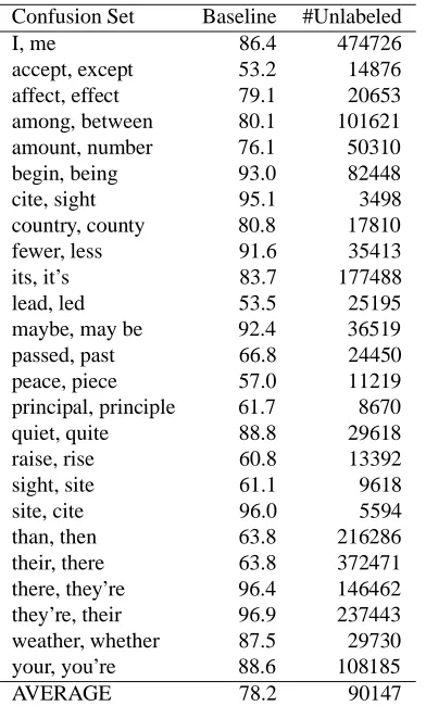
Table 1: Confusion Sets used in the Experiments
Confusion Set Baseline #Unlabeled
I, me 86.4 474726
accept, except 53.2 14876 affect, effect 79.1 20653 among, between 80.1 101621 amount, number 76.1 50310
begin, being 93.0 82448
cite, sight 95.1 3498
country, county 80.8 17810
fewer, less 91.6 35413
its, it’s 83.7 177488
lead, led 53.5 25195
maybe, may be 92.4 36519
passed, past 66.8 24450
peace, piece 57.0 11219
principal, principle 61.7 8670
quiet, quite 88.8 29618
raise, rise 60.8 13392
sight, site 61.1 9618
site, cite 96.0 5594
than, then 63.8 216286
their, there 63.8 372471
there, they’re 96.4 146462 they’re, their 96.9 237443 weather, whether 87.5 29730
your, you’re 88.6 108185
AVERAGE 78.2 90147
5
Experiment
To conduct large scale experiments, we used the British National Corpus1that is currently one of the largest cor-pora available. The corpus contains roughly one hundred million words collected from various sources.
The confusion sets used in our experiments are the same as in Golding’s experiment (1999). Since our al-gorithm requires the classification to be binary, we de-composed three-class confusion sets into pairwise binary classifications. Table 1 shows the resulting confusion sets used in the following experiments. The baseline perfor-mances, achieved by simply selecting the majority class, are shown in the second column. The number of unla-beled data are shown in the rightmost column.
The 1,000 test sets were randomly selected from the corpus for each confusion set. They do not overlap the labeled data or the unlabeled data used in the learning process.
1
[image:4.612.318.535.107.444.2]Data cited herein has been extracted from the British Na-tional Corpus Online service, managed by Oxford University Computing Services on behalf of the BNC Consortium. All rights in the texts cited are reserved.
Table 2: Results of Confusion Sets Disambiguation with 32 Labeled Data
NB + EM
Confusion Set NB NB+EM +CDC
I, me 87.4 96.3 96.0
accept, except 77.2 89.0 81.1 affect, effect 86.4 91.6 93.6 among, between 80.1 64.4 79.5 amount, number 69.6 61.6 68.8
begin, being 95.1 86.6 95.1
cite, sight 95.1 95.1 95.1
country, county 77.5 70.4 76.0
fewer, less 89.0 77.4 85.4
its, it’s 85.3 92.3 94.2
lead, led 65.3 64.2 63.7
maybe, may be 91.1 77.6 92.9
passed, past 77.9 70.2 82.0
peace, piece 78.4 81.5 82.1
principal, principle 72.8 88.7 79.4
quiet, quite 85.3 75.9 83.5
raise, rise 83.7 86.1 81.0
sight, site 67.7 68.7 67.9
site, cite 96.2 93.3 92.8
than, then 74.7 84.0 85.3
their, there 88.4 91.4 90.2
there, they’re 96.4 96.4 89.1 they’re, their 96.9 96.9 96.9 weather, whether 90.6 92.3 93.7
your, you’re 87.8 81.8 90.3
AVERAGE 83.8 82.9 85.4
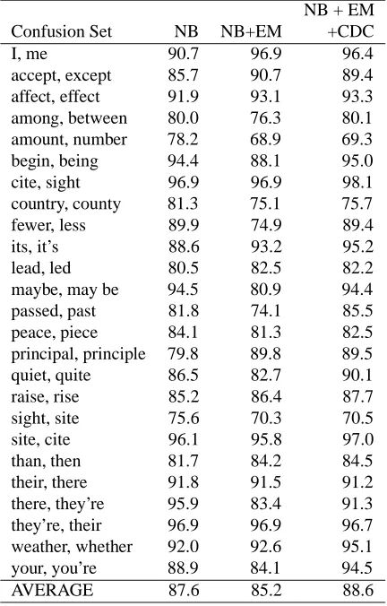
The results are shown in Table 2 through Table 5. These four tables correspond to the cases in which the number of labeled examples is 32, 64, 128 and 256 as indicated by the table captions. The first column shows the confusion sets. The second column shows the clas-sification performance of the naive Bayes classifier with which only labeled data was used for training. The third column shows the performance of the naive Bayes classi-fier with which unlabeled data was used via the basic EM algorithm. The rightmost column shows the performance of the EM algorithm that was extended with our proposed calibration process.
Notice that the effect of unlabeled data were very dif-ferent for each confusion set. As shown in Table 2, the precision was significantly improved for some confusion sets including{I, me},{accept, except}and{affect, ef-fect} . However, disastrous performance deterioration can be observed, especially that of the basic EM algo-rithm, in some confusion sets including {among, be-tween},{country, county}, and{site, cite}.
un-Table 3: Results of Confusion Sets Disambiguation with 64 Labeled Data
NB + EM
Confusion Set NB NB+EM +CDC
I, me 89.4 96.8 95.7
accept, except 82.9 89.3 87.5 affect, effect 89.4 92.4 93.6 among, between 79.9 76.3 80.5 amount, number 71.5 68.7 69.1
begin, being 95.8 92.1 95.7
cite, sight 95.1 95.8 96.4
country, county 78.7 73.4 74.5
fewer, less 87.6 74.3 87.3
its, it’s 85.8 94.0 92.5
lead, led 76.2 66.8 72.8
maybe, may be 92.6 84.0 96.2
passed, past 79.7 72.5 88.4
peace, piece 81.1 81.2 82.4
principal, principle 75.2 90.2 89.8
quiet, quite 86.5 84.0 89.2
raise, rise 85.7 85.6 86.9
sight, site 71.9 69.0 69.0
site, cite 96.3 95.8 95.5
than, then 79.7 83.8 83.2
their, there 90.5 91.9 92.1
there, they’re 96.2 85.2 91.4 they’re, their 96.9 96.9 95.8 weather, whether 90.6 91.4 93.3
your, you’re 88.0 83.3 94.2
AVERAGE 85.7 84.6 87.7
labeled data via the basic EM algorithm (from 83.3% to 82.9%). On the other hand, the EM algorithm with the class distribution constraint improved average classifica-tion performance (from 83.3% to 85.4%). This improved precision nearly reached the performance achieved by twice the size of labeled data without unlabeled data (see the average precision of NB in Table 3). This perfor-mance gain indicates that the use of unlabeled data ef-fectively doubles the labeled training data.
In Table 3, the tendency of performance improvement (or degradation) in the use of unlabeled data is almost the same as in Table 2. The basic EM algorithm degraded the performance on average, while our method improved av-erage performance (from 85.7% to 87.7%). This perfor-mance gain effectively doubled the size of labeled data.
The results with 128 labeled examples are shown in Ta-ble 4. Although the use of unlabeled examples by means of our proposed method still improved average perfor-mance (from 87.6% to 88.6%), the gain is smaller than that for a smaller amount of labeled data.
With 256 labeled examples (Table 5), the average
per-Table 4: Results of Confusion Sets Disambiguation with 128 Labeled Data
NB + EM
Confusion Set NB NB+EM +CDC
I, me 90.7 96.9 96.4
accept, except 85.7 90.7 89.4 affect, effect 91.9 93.1 93.3 among, between 80.0 76.3 80.1 amount, number 78.2 68.9 69.3
begin, being 94.4 88.1 95.0
cite, sight 96.9 96.9 98.1
country, county 81.3 75.1 75.7
fewer, less 89.9 74.9 89.4
its, it’s 88.6 93.2 95.2
lead, led 80.5 82.5 82.2
maybe, may be 94.5 80.9 94.4
passed, past 81.8 74.1 85.5
peace, piece 84.1 81.3 82.5
principal, principle 79.8 89.8 89.5
quiet, quite 86.5 82.7 90.1
raise, rise 85.2 86.4 87.7
sight, site 75.6 70.3 70.5
site, cite 96.1 95.8 97.0
than, then 81.7 84.2 84.5
their, there 91.8 91.5 91.2
there, they’re 95.9 83.4 91.3 they’re, their 96.9 96.9 96.7 weather, whether 92.0 92.6 95.1
your, you’re 88.9 84.1 94.5
AVERAGE 87.6 85.2 88.6
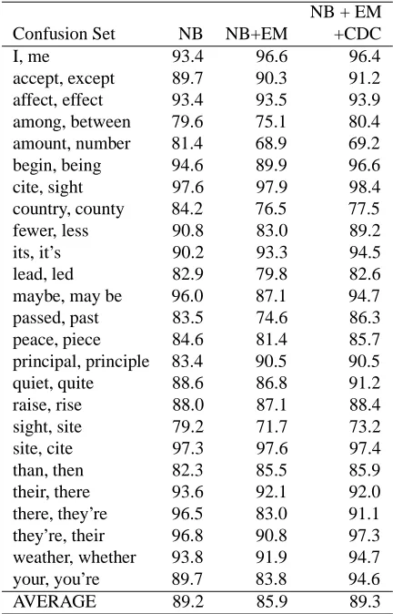
formance gain was negligible (from 89.2% to 89.3%). Figure 1 summarizes the average precisions for differ-ent number of labeled examples. Average peformance was improved by the use of unlabeled data with our pro-posed method when the amount of labeled data was small (from 32 to 256) as shown in Table 2 through Table 5. However, when the number of labeled examples was large (more than 512), the use of unlabeled data degraded average performance.
5.1 Effect of the amount of unlabeled data
When the use of unlabeled data improves classification performance, the question of how much unlabeled data are needed becomes very important. Although unlabeled data are generally much more obtainable than labeled data, acquiring more than several-thousand unlabeled ex-amples is not always an easy task. As for confusion set disambiguation, Table 1 indicates that it is sometimes im-possible to collect tens of thousands examples even in a very large corpus.
[image:5.612.78.296.106.444.2] [image:5.612.319.535.107.445.2]un-Table 5: Results of Confusion Sets Disambiguation with 256 Labeled Data
NB + EM
Confusion Set NB NB+EM +CDC
I, me 93.4 96.6 96.4
accept, except 89.7 90.3 91.2 affect, effect 93.4 93.5 93.9 among, between 79.6 75.1 80.4 amount, number 81.4 68.9 69.2
begin, being 94.6 89.9 96.6
cite, sight 97.6 97.9 98.4
country, county 84.2 76.5 77.5
fewer, less 90.8 83.0 89.2
its, it’s 90.2 93.3 94.5
lead, led 82.9 79.8 82.6
maybe, may be 96.0 87.1 94.7
passed, past 83.5 74.6 86.3
peace, piece 84.6 81.4 85.7
principal, principle 83.4 90.5 90.5
quiet, quite 88.6 86.8 91.2
raise, rise 88.0 87.1 88.4
sight, site 79.2 71.7 73.2
site, cite 97.3 97.6 97.4
than, then 82.3 85.5 85.9
their, there 93.6 92.1 92.0
there, they’re 96.5 83.0 91.1 they’re, their 96.8 90.8 97.3 weather, whether 93.8 91.9 94.7
your, you’re 89.7 83.8 94.6
AVERAGE 89.2 85.9 89.3
labeled data, we conducted experiments by varying the amount of unlabeled data for some confusion sets that ex-hibited significant performance gain by using unlabeled data.
Figure 2 shows the relationship between the classifica-tion performance and the amount of unlabeled data for three confusion sets:{I, me},{principal, principle}, and {passed, past}. The number of labeled examples in all cases was 64.
Note that performance continued to improve even when the number of unlabeled data reached more than ten thousands. This suggests that we can further improve the performance for some confusion sets by using a very large corpus containing more than one hundred million words.
Figure 2 also indicates that the use of unlabeled data was not effective when the amount of unlabeled data was smaller than one thousand. It is often the case with mi-nor words that the number of occurrences does not reach one thousand even in a one-hundred-million word corpus. Thus, constructing a very very large corpus (containing
75 80 85 90 95 100
100 1000
Precision (%)
[image:6.612.320.542.76.237.2]Number of Labeled Examples NB NB+EM NB+EM+CDC
Figure 1: Relationship between Average Precision and the Amount of Labeled Data
60 65 70 75 80 85 90 95 100
1000 10000 100000
Precision (%)
Number of Unlabeled Examples I, me principal, principle passed, past
Figure 2: Relationship between Precision and the Amount of Unlabeled Data
more than billions of words) appears to be beneficial for infrequent words.
6
Related Work
Nigam et al.(2000) reported that the accuracy of text clas-sification can be improved by a large pool of unlabeled documents using a naive Bayes classifier and the EM al-gorithm. They presented two extensions to the basic EM algorithm. One is a weighting factor to modulate the con-tribution of the unlabeled data. The other is the use of multiple mixture components per class. With these exten-sions, they reported that the use of unlabeled data reduces classification error by up to 30%.
[image:6.612.77.293.106.443.2] [image:6.612.318.537.288.446.2]per-formance on average. The amount of unlabeled data used in their experiments was relatively small (from several hundreds to a few thousands).
Yarowsky (1995) presented an approach that signif-icantly reduces the amount of labeled data needed for word sense disambiguation. Yarowsky achieved accura-cies of more than 90% for two-sense polysemous words. This success was likely due to the use of “one sense per discourse” characteristic of polysemous words.
Yarowsky’s approach can be viewed in the context of co-training (Blum and Mitchell, 1998) in which the fea-tures can be split into two independent sets. For word sense disambiguation, the sets correspond to the local contexts of the target word and the “one sense per dis-course” characteristic. Confusion sets however do not have the latter characteristic.
The effect of a huge amount of unlabeled data for confusion set disambiguation is discussed in (Banko and Brill, 2001). Bank and Brill conducted experiments of committee-based unsupervised learning for two confu-sion sets. Their results showed that they gained a slight improvement by using a certain amount of unlabeled data. However, test set accuracy began to decline as ad-ditional data were harvested.
As for the performance of confusion set disambigua-tion, Golding (1999) achieved over 96% by a winnow-based approach. Although our results are not directly comparable with their results since the data sets are different, our results does not reach the state-of-the-art performance. Because the performance of a naive Bayes classifier is significantly affected by the smoothing method used for paramter estimation, there is a chance to improve our performance by using a more sophisticated smoothing technique.
7
Conclusion
The naive Bayes classifier can be combined with the well-established EM algorithm to exploit the unlabeled data . However, the use of unlabeled data sometimes causes disastrous degradation of classification performance.
In this paper, we introduce a class distribution con-straint into the iteration process of the EM algorithm. This constraint keeps the class distribution of unlabeled data consistent with the true class distribution estimated from labeled data, preventing the EM algorithm from converging into an undesirable state.
Experimental results using 26 confusion sets and a large amount of unlabeled data showed that combining the EM algorithm with our proposed constraint consis-tently reduced the average classification error rates when the amount of labeled data is small. The results also showed that use of unlabeled data is especially advan-tageous when the amount of labeled data is small (up to about one hundred).
7.1 Future Work
In this paper, we empirically demonstrated that a class distribution constraint reduced the chance of undesirable convergence of the EM algorithm. However, the theoret-ical justification of this constraint should be clarified in future work.
References
Michele Banko and Eric Brill. 2001. Scaling to very very large corpora for natural language disambiguation. In Proceedings of the Association for Computational Lin-guistics.
Adam L. Berger, Stephen A. Della Pietra, and Vincent J. Della Pietra. 1996. A maximum entropy approach to natural language processing. Computational Linguis-tics, 22(1):39–71.
Avrim Blum and Tom Mitchell. 1998. Combin-ing labeled and unlabeled data with co-trainCombin-ing. In COLT: Proceedings of the Workshop on Computa-tional Learning Theory, Morgan Kaufmann Publish-ers.
Michael Collins and Yoram Singer. 1999. Unsupervised models for named entity classification. In Proceedings of the Joint SIGDAT Conference on Empirical Meth-ods in Natural Language Processing and Very Large Corpora.
A. P. Dempster, N. M. Laird, and D. B. Rubin. 1977. Maximum likelihood from incomplete data via the em algorithm. Royal Statstical Society B 39, pages 1–38.
G. Escudero, L. arquez, and G. Rigau. 2000. Naive bayes and exemplar-based approaches to word sense disam-biguation revisited. In Proceedings of the 14th Euro-pean Conference on Artificial Intelligence.
Andrew R. Golding and Dan Roth. 1999. A winnow-based approach to context-sensitive spelling correc-tion. Machine Learning, 34(1-3):107–130.
Thorsten Joachims. 1999. Transductive inference for text classification using support vector machines. In Proc. 16th International Conf. on Machine Learning, pages 200–209. Morgan Kaufmann, San Francisco, CA.
David D. Lewis. 1998. Naive Bayes at forty: The in-dependence assumption in information retrieval. In Claire N´edellec and C´eline Rouveirol, editors, Pro-ceedings of ECML-98, 10th European Conference on Machine Learning, number 1398, pages 4–15, Chem-nitz, DE. Springer Verlag, Heidelberg, DE.
Andrew McCallum and Kamal Nigam. 1998. A com-parison of event models for naive bayes text classifica-tion. In AAAI-98 Workshop on Learning for Text Cat-egorization.
Kamal Nigam and Rayid Ghani. 2000. Analyzing the ef-fectiveness and applicability of co-training. In CIKM, pages 86–93.
Kamal Nigam, Andrew Kachites Mccallum, Sebastian Thrun, and Tom Mitchell. 2000. Text classification from labeled and unlabeled documents using EM. Ma-chine Learning, 39(2/3):103–134.
Ted Pedersen and Rebecca Bruce. 1998. Knowledge lean word-sense disambiguation. In AAAI/IAAI, pages 800–805.
Ted Pedersen. 2000. A simple approach to building en-sembles of naive bayesian classifiers for word sense disambiguation. In Proceedings of the First Annual Meeting of the North American Chapter of the Asso-ciation for Computational Linguistics, pages 63–69, Seattle, WA, May.
David M. W. Powers. 1998. Learning and application of differential grammars. In T. Mark Ellison, editor, CoNLL97: Computational Natural Language Learn-ing, pages 88–96. Association for Computational Lin-guistics, Somerset, New Jersey.
Adwait Ratnaparkhi. 1998. Maximum Entropy Models for Natural Language Ambiguity Resolution. Ph.D. thesis, the University of Pennsylvania.
Robert E. Schapire and Yoram Singer. 2000. Boostex-ter: A boosting-based system for text categorization. Machine Learning, 39(2/3):135–168.
Vladimir N. Vapnik. 1995. The Nature of Statistical Learning Theory. New York.
David Yarowsky. 1994. Decision lists for lexical ambi-guity resolution: Application to accent restoration in spanish and french. In Meeting of the Association for Computational Linguistics, pages 88–95.