A Weakly Supervised Model for Sentence-Level Semantic Orientation
Analysis with Multiple Experts
Lizhen Qu and Rainer Gemulla and Gerhard Weikum Max Planck Institute for Informatics
Saarbr¨ucken, Germany
{lqu,rgemulla,weikum}@mpi-inf.mpg.de
Abstract
We propose the weakly supervised Multi-Experts Model (MEM) for analyzing the se-mantic orientation of opinions expressed in natural language reviews. In contrast to most prior work, MEM predicts both opinion po-larity and opinion strength at the level of in-dividual sentences; such fine-grained analysis helps to understand better why users like or dislike the entity under review. A key chal-lenge in this setting is that it is hard to ob-tain sentence-level training data for both po-larity and strength. For this reason, MEM is weakly supervised: It starts with potentially noisy indicators obtained from coarse-grained training data (i.e., document-level ratings), a small set of diverse base predictors, and, if available, small amounts of fine-grained train-ing data. We integrate these noisy indicators into a unified probabilistic framework using ideas from ensemble learning and graph-based semi-supervised learning. Our experiments in-dicate that MEM outperforms state-of-the-art methods by a significant margin.
1 Introduction
Opinion mining is concerned with analyzing opin-ions expressed in natural language text. For example, many internet websites allow their users to provide both natural language reviews and numerical ratings to items of interest (such as products or movies). In this context, opinion mining aims to uncover the relationship between users and (features of) items. Preferences of users to items can be well understood by coarse-grained methods of opinion mining, which
focus on analyzing the semantic orientation of doc-uments as a whole. To understandwhyusers like or dislike certain items, however, we need to perform more fine-grained analysis of the review text itself.
In this paper, we focus on sentence-level analy-sis of semantic orientation (SO) in online reviews. The SO consists of polarity(positive, negative, or other1) andstrength(degree to which a sentence is positive or negative). Both quantities can be ana-lyzed jointly by mapping them to numerical ratings: Large negative/positive ratings indicate a strong neg-ative/positive orientation. A key challenge in fine-grained rating prediction is that fine-fine-grained train-ing data for both polarity and strength is hard to obtain. We thus focus on a weakly supervised set-ting in which only coarse-level training data (such as document ratings and subjectivity lexicons) and, optionally, a small amount of fine-grained training data (such as sentence polarities) is available.
A number of lexicon-based approaches for phrase-level rating prediction has been proposed in the liter-ature (Taboada et al., 2011; Qu et al., 2010). These methods utilize a subjectivity lexicon of words along with information about their semantic orientation; they focus on phrases that contain words from the lexicon. A key advantage of sentence-level methods is that they are able to cover all sentences in a review and that phrase identification is avoided. To the best of our knowledge, the problem of rating prediction at the sentence level has not been addressed in the literature. A naive approach would be to simply aver-age phrase-level ratings. Such an approach performs
1We assign polarityotherto text fragments that are off-topic
or not directly related to the entity under review.
poorly, however, since (1) phrases are analyzed out of context (e.g., modal verbs or conditional clauses), (2) domain-dependent information about semantic orientation is not captured in the lexicons, (3) only phrases that contain lexicon words are covered. Here (1) and (2) lead to low precision, (3) to low recall.
To address the challenges outlined above, we pro-pose the weakly supervised Multi-Experts Model (MEM) for sentence-level rating prediction. MEM starts with a set of potentially noisy indicators of SO including phrase-level predictions, language heuris-tics, and co-occurrence counts. We refer to these indicators asbase predictors; they constitute the set of experts used in our model. MEM is designed such that new base predictors can be easily integrated. Since the information provided by the base predictors can be contradicting, we use ideas from ensemble learning (Dietterichl, 2002) to learn the most con-fident indicators and to exploit domain-dependent information revealed by document ratings. Thus, in-stead of averaging base predictors, MEM integrates their features along with the available coarse-grained training data into a unified probabilistic model.
The integrated model can be regarded as a Gaus-sian process (GP) model (Rasmussen, 2004) with a novel multi-expert prior. The multi-expert prior decomposes into two component distributions. The first component distribution integrates sentence-local information obtained from the base predictors. It forms a special realization of stacking (Dzeroski and Zenko, 2004) but uses the features from the base pre-dictors instead of the actual predictions. The second component distribution propagates SO information across similar sentences using techniques from graph-based semi-supervised learning (GSSL) (Zhu et al., 2003; Belkin et al., 2006). It aims to improve the predictions on sentences that are not covered well enough by our base predictors. Traditional GSSL al-gorithms support either discrete labels (classification) or numerical labels (regression); we extend these techniques to support both types of labels simulta-neously. We use a novel variant of word sequence kernels (Cancedda et al., 2003) to measure sentence similarity. Our kernel takes the relative positions of words but also their SO and synonymity into account.
Our experiments indicate that MEM significantly outperforms prior work in both sentence-level rating prediction and sentence-level polarity classification.
2 Related Work
There exists a large body of work on analyzing the semantic orientation of natural language text. Our approach is unique in that it is weakly supervised, predicts both polarity and strength, and operates on the sentence level.
Supervised approaches for sentiment analysis fo-cus mainly on opinion mining at the document level (Pang and Lee, 2004; Pang et al., 2002; Pang and Lee, 2005; Goldberg and Zhu, 2006), but have also been applied to sentence-level polarity classifi-cation in specific domains (Mao and Lebanon, 2006; Pang and Lee, 2004; McDonald et al., 2007). In these settings, a sufficient amount of training data is available. In contrast, we focus on opinion mining tasks with little or no fine-grained training data.
The weakly supervised HCRF model (T¨ackstr¨om and McDonald, 2011b; T¨ackstr¨om and McDonald, 2011a) for sentence-level polarity classification is per-haps closest to our work in spirit. Similar to MEM, HCRF uses coarse-grained training data and, when available, a small amount of fine-grained sentence polarities. In contrast to MEM, HCRF does not pre-dict the strength of semantic orientation and ignores the order of words within sentences.
There exists a large number of lexicon-based meth-ods for polarity classification (Ding et al., 2008; Choi and Cardie, 2009; Hu and Liu, 2004; Zhuang et al., 2006; Fu and Wang, 2010; Ku et al., 2008). The lexicon-based methods of (Taboada et al., 2011; Qu et al., 2010) also predict ratings at the phrase level; these methods are used as experts in our model.
MEM leverages ideas from ensemble learning (Di-etterichl, 2002; Bishop, 2006) and GSSL meth-ods (Zhu et al., 2003; Zhu and Ghahramani, 2002; Chapelle et al., 2006; Belkin et al., 2006). We extend GSSL with support for multiple, heterogenous labels. This allows us to integrate our base predictors as well as the available training data into a unified model that exploits that strengths of algorithms from both families.
3 Base Predictors
(see Sec. 4.4). MEM is designed such that new base predictors can be integrated easily.
Our base predictors use a diverse set of available web and linguistic resources. The hope is that this di-versity increases overall prediction performance (Di-etterichl, 2002): Thestatistical polarity predictor fo-cuses on local syntactic patterns; it is based on corpus statistics for SO-carrying words and opinion topic words. Theheuristic polarity predictoruses manu-ally constructed rules to achieve high precision but low recall. Both thebag-of-opinions rating predictor and theSO-CAL rating predictorare based on lexi-cons. The BoO predictor uses a lexicon trained from a large generic-domain corpus and is recall-oriented; the SO-CAL predictor uses a different lexicon with manually assigned weights and is precision-oriented.
3.1 Statistical Polarity Predictor
The polarity of an SO-carrying word strongly de-pends on its target word. For example, consider the phrase “I began this novel with thegreatestofhopes [...]”. Here, “greatest” has a positive semantic orien-tation in all subjectivity lexicons, but the combination “greatest of hopes” often indicates a negative
senti-ment. We refer to a pair of SO-carrying word (“great-est”) and a target word (“hopes”) as anopinion-target pair. Our statistical polarity predictor learns the po-larity of opinions and targets jointly, which increases the robustness of its predictions.
Syntactic dependency relations of the form
A −R→ B are a strong indicator for opinion-target pairs (Qiu et al., 2009; Zhuang et al., 2006); e.g., “great”−−−→nmod “product”. To achieve high precision, we only consider pairs connected by the follow-ing predefined set of shortest dependency paths:
verb ←−−subj noun, verb ←−obj noun, adj −−−→nmod noun,
adj −prd−→ verb ←−−subj noun. We only retain opinion-target pairs that are sufficiently frequent.
For each extracted pairz, we count how often it co-occurs with each document polarityy∈ Y, where Y ={positive,negative,other}denotes the set of po-larities. Ifzoccurs in a document but is preceded by a negator, we treat it as a co-occurrence of opposite document polarity. Ifzoccurs in a document with po-larityother, we count the occurrence with only half weight, i.e., we increase both #z and #(other, z)
by 0.5. These documents are typically a mixture of
positive and negative opinions so that we want to reduce their impact. The marginal distribution of polarity labelygiven thatzoccurs in a sentence is estimated asP(y|z) = #(y, z)/#z. The predictor is trained using the text and ratings of the reviews in the training data, i.e., without relying on fine-grained annotations.
The statistical polarity predictor can be used to pre-dict sentence-level polarities by averaging the phrase-level predictions. As discussed previously, such an approach is problematic; we use it as a baseline ap-proach in our experimental study. We also employ phrase-level averaging to estimate the variance of base predictors; see Sec. 4.3. Denote byZ(x)the set of opinion-target pairs in sentencex. To predict the sentence polarityy ∈ Y, we take the Bayesian aver-age of the phrase-level predictors: P(y | Z(x)) =
P
z∈Z(x)P(y | z)P(z) = P
z∈Z(x)P(y, z). Thus the most likely polarity is the one with the highest co-occurrence count.
3.2 Heuristic Polarity Predictor
Heuristic patterns can also serve as base predictors. In particular, we found that some authors list positive and negative aspects separately after keywords such as “pros” and “cons”. A heuristic that exploits such patterns achieved a high precision (>90%) but low recall (<5%) in our experiments.
3.3 Bag-of-Opinions Rating Predictor
We leverage the bag-of-opinion (BoO) model of Qu et al. (2010) as a base predictor for phrase-level ratings. The BoO model was trained from a large generic corpus without fine-grained annotations.
In BoO, an opinion consists of three components: an SO-carrying word (e.g., “good”), a set of intensi-fiers (e.g., “very”) and a set of negators (e.g., “not”). Each opinion is scored based on these words (repre-sented as a boolean vectorb) and the polarity of the SO-carrying word (represented assgn(r)∈ {−1,1}) as indicated by the MPQA lexicon of Wilson et al. (2005). In particular, the score is computed as
word, respectively.
3.4 SO-CAL Rating Predictor
The Semantic Orientation Calculator (SO-CAL) of Taboada et al. (2011) also predicts phrase-level rat-ings via a scoring function similar to the one of BoO. The SO-CAL predictor uses a manually created lexi-con, in which each word is classified as either an SO-carrying word (associated with a numerical score), an intensifier (associated with a modifier on the numer-ical score), or a negator. SO-CAL employs various heuristics to detect irrealis and to correct for the pos-itive bias inherent in most lexicon-based classifiers. Compared to BoO, SO-CAL has lower recall but higher precision.
4 Multi-Experts Model
Our multi-experts model incorporates features from the individual base predictors, coarse-grained labels (i.e., document ratings or polarities), similarities be-tween sentences, and optionally a small amount of sentence polarity labels into an unified probabilistic model. We first give an overview of MEM, and then describe its components in detail.
4.1 Model Overview
Denote by X = {x1, . . . ,xN} a set of sentences. We associate each sentencexi with a set ofinitial
labelsyiˆ, which are strong indicators of semantic orientation: the coarse-grained rating of the corre-sponding document, the polarity label of our heuristic polarity predictor, the phrase-level ratings from the SO-CAL predictor, and optionally a manual polarity label. Note that the number of initial labels may vary from sentence to sentence and that initial labels are heterogeneous in that they refer to either polarities or ratings. LetYˆ = {yˆ1, . . . ,ˆyN}. Our goal is to predict the unobserved ratingsr={r1, . . . , rN}of each sentence.
Our multi-expert model is a probabilistic model forX,Yˆ, andr. In particular, we model the rating vectorrvia a multi-expert priorPE(r|X,β)with
parameterβ(Sec. 4.2).PEintegrates both features
from the base predictors and sentence similarities. We correlate ratings to initial labels via a set of con-ditional distributionsPb(ˆyb|r), wherebdenotes the type of initial label (Sec. 4.3). The posterior ofris
then given by
P(r|X,Yˆ,β)∝Y
b
Pb(ˆyb |r)PE(r|X,β).
Note that the posterior is influenced by both the multi-expert prior and the set of initial labels.
We use MAP inference to obtain the most likely rating of each sentence, i.e., we solve
argmin
r,β
−X
b
log(Pb(yˆb |r))−log(PE(r|X,β)),
where as beforeβdenotes the model parameters. We solve the above optimization problem using cyclic coordinate descent (Friedman et al., 2008).
4.2 Multi-Expert Prior
The multi-expert priorPE(r|X,β)consists of two
component distributions N1 and N2. Distribution N1integrates features from the base predictors,N2 incorporates sentence similarities to propagate infor-mation across sentences.
In a slight abuse of notation, denote byxithe set of features for thei-th sentence. Vectorxi contains the features of all the base predictors but also includes bi-gram features for increased coverage of syntactic pat-terns; see Sec. 4.4 for details about the feature design. Letm(xi) =βTxibe a linear predictor forri, where βis a real weight vector. Assuming Gaussian noise,
ri follows a Gaussian distributionN1(ri | mi, σ2) with meanmi =m(xi)and varianceσ2. Note that predictormcan be regarded as a linear combination of base predictors because bothmand each of the base predictors are linear functions. By integrating all features into a single function, the base predictors are trained jointly so that weight vectorβ automati-cally adapts to domain-dependent properties of the data. This integrated approach significantly outper-formed the alternative approach of using a weighted vote of the individual predictions made by the base predictors. We regularize the weight vectorβ us-ing a Laplace priorP(β | α) with parameterα to encourage sparsity.
like to capture sentence similarity using gapped (i.e., non-consecutive) subsequences. For example, the sentences “The book is an easy read.” and “It is easy to read.” are similar but do not share any consecutive bigrams. They do share the subsequence “easy read”, however. To capture this similarity, we make use of a novel sentiment-augmented variant of word sequence kernels (Cancedda et al., 2003). Our kernel is used to construct a similarity matrixWamong sentences and the corresponding regularized LaplacianLe. To capture the intuition that similar sentences should have similar ratings, we introduce a Gaussian prior N2(r|0,Le−1)as a component into our multi-expert prior; see Sec. 4.5 for details and a discussion of why this prior encourages similar ratings for similar sentences.
Since the two component distributions feature dif-ferent expertise, we take their product and obtain the multi-expert prior
PE(r|X,β)∝ N1(r|m,Iσ2)N2(r|0,Le−1)P(β|α),
wherem = (m1, . . . , mN). Note that the normal-izing constant of PE can be ignored during MAP
inference since it does not depend onβ.
4.3 Incorporating Initial Labels
Recall that the initial labels Yˆ are strong indica-tors of semantic orientation associated with each sentence; they correspond to either discrete polarity labels or to continuous rating labels. This hetero-geneity constitutes the main difficulty for incorporat-ing the initial labels via the conditional distributions
Pb(ˆyb |r). We assume independence throughout so thatPb(ˆyb |r) =
Q
iPb(ˆyib|ri).
Rating Labels For continuous labels, we assume Gaussian noise and setPb(ˆyib |ri) =N(ˆybi |ri, ηib), where varianceηbi is a type- and sentence-dependent. For SO-CAL labels, we simply set ηiSO-CAL = ηSO-CAL, whereηSO-CAL is a hyperparameter. The SO-CAL scores have limited influence in our overall model; we found that more complex designs lead to little improvement. We proceed differently for docu-ment ratings. Our experidocu-ment suggests that docudocu-ment ratings constitute the most important indicator of the SO of a sentence. Thus sentence ratings should be close to document ratings unless strong evidence to
the contrary exists. In other words, we want variance
ηiDocto be small.
When no manually created sentence-level polar-ity labels are available, we set the value ofηDoci de-pending on the polarity class. In particular, we set
ηDoc
i = 1for both positive and negative documents, andηiDoc= 2for neutral documents. The reasoning behind this choice is that sentence ratings in neu-tral documents express higher variance because these documents often contain a mixture of positive and negative sentences.
When a small set of manually created sentence polarity labels is available, we train a classifier that predicts whether the sentence polarity coincides with the document polarity. If so, we set the corresponding varianceηDoci to a small value; otherwise, we choose a larger value. In particular, we train a logistic regres-sion classifier (Bishop, 2006) using the following binary features: (1) an indicator variable for each document polarity, and (2) an indicator variable for each triple of base predictor, predicted polarity, and document polarity (set to1if the polarities match). We then setηiDoc= (τ pi)−1, wherepiis the probabil-ity of matching polarities obtained from the classifier andτ is a hyperparameter that ensures correct scal-ing.
Polarity Labels We now describe how to model the correlation between the polarity of a sentence and its rating. An simple and effective approach is to partition the range of ratings into three consecutive partitions, one for each polarity class. We thus consid-ering the polarity classes{positive,other,negative} as ordered and formulate polarity classification as an ordinal regression problem (Chu and Ghahramani, 2006). We immediately obtain the distribution
Pb(ˆyib=pos|ri) = Φ
ri−b+
p
ηb
!
Pb(ˆybi =oth|ri) = Φ
b+−ri
p
ηb
!
−Φ b
−−r i
p
ηb
!
Pb(ˆybi =neg|ri) = Φ
b−−ri
p
ηb
!
,
whereb+andb−are the partition boundaries between positive/otherandother/negative, respectively,2Φ(x)
denotes the cumulative distribution function of the
2We setb+
Figure 1: Distribution of polarity given rating.
Gaussian distribution, and variance ηb is a hyper-parameter. It is easy to verify that P
ˆ yb
i∈Yp(ˆy
b i |
ri) = 1. The resulting distribution is shown in Fig. 1. We can use the same distribution to use MEM for sentence-level polarity classification; in this case, we pick the polarity with the highest probability.
4.4 Incorporating Base Predictors
Base predictors are integrated into MEM via compo-nentN1(ri | mi, σ2) of the multi-expert prior (see Sec. 4.2). Recall thatmi is a linear function of the featuresxi of each sentence. In this section, we dis-cuss howxiis constructed from the features of the base predictors. New base predictors can be inte-grated easily by exposing their features to MEM.
Most base predictors operate on the phrase level; our goal is to construct features for the entire sen-tence. Denote by nbi the number of phrases in the
i-th sentence covered by base predictor b, and let obij denote a set of associated features. Featuresobij may or may not correspond directly to the features of base predictor b; see the discussion below. A straightforward strategy is to setxbi = (nbi)−1P
jobij. We proceed slightly differently and average the fea-tures associated with phrases of positive prior polar-ity separately from those of phrases with negative prior polarity (Taboada et al., 2011). We then con-catenate the averaged feature vectors, i.e., we set xbi = (¯ob,posij o¯b,negij ), whereo¯b,pij denotes the average of the feature vectorsobij associated with phrases of prior polarityp. This procedure allows us to learn a different weight for each feature depending on its
context (e.g., the weight of intensifier “very” may dif-fer for positive and negative phrases). We construct xiby concatenating the sentence-level featuresxbi of each base predictor and a feature vector of bigrams. To integrate a base predictor, we only need to specify the relevant features and, if applicable, prior phrase polarities. For our choice of base predictors, we use the following features:
SO-CAL predictor. The prior polarity of a CAL phrase is given by the polarity of its SO-carrying word in the SO-CAL lexicon. The feature vector oSO-CALij consists of the weight of the SO-carrying word from the lexicon as well the set of negator words, irrealis marker words, and intensifier words in the phrase. Moreover, we add the first two words preceding the SO-carrying word as context features (skipping nouns, negators, irrealis markers, and intensifiers, and stopping at clause boundaries). All words are encoded as binary indicator features.
BoO predictor. Similar to SO-CAL, we deter-mine the prior polarity of a phrase based on the BoO dictionary. In contrast to SO-CAL, we directly use the BoO score as a feature because the BoO predictor weights have been trained on a very large corpus and are thus reliable. We also add irrealis marker words in the form of indicator features.
Statistical polarity predictor. Recall that the sta-tistical polarity predictor is based on co-occurrence counts of opinion-topic pairs and document polar-ities. We treat each opinion-topic pair as a phrase and use the most frequently co-occurring polarity as the phrase’s prior polarity. We use the logarithm of the co-occurrence counts with positive, negative, and other polarity as features; this set of features per-formed better than using the co-occurrence counts or estimated class probabilities directly. We also add the same type of context features as for SO-CAL, but rescale each binary feature by the logarithm of the occurrence count#zof the opinion-topic pair (i.e., the features take values in{0,log #z}).
4.5 Incorporating Sentence Similarities
be-cause they do not contain SO-carrying words). To obtain this distribution, we first construct anN ×N
sentence similarity matrix W using a sentiment-augmented word sequence kernel (see below). We then compute the regularized graph LaplacianLe = L+I/λ2based on the unnormalized graph Laplacian L=D−W(Chapelle et al., 2006), whereDbe a diagonal matrix withdii=Pjwij and hyperparam-eterλ2controls the scale of sentence ratings.
To gain insight into distributionN2, observe that
N2(r|0,Le−1)
∝exp
−1
2
X
i,j
wij(ri−rj)2− krk22/λ2
.
The left term in the exponent forces the ratings of similar sentences to be similar: the larger the sen-tence similaritywij, the more penalty is paid for dis-similar ratings. For this reason,N2 has a smoothing effect. The right term is an L2 regularizer and encour-ages small ratings; it is controlled by hyperparameter
λ2.
The entrieswij in the sentence similarity matrix determine the degree of smoothing for each pair of sentence ratings. We compute these values by a novel sentiment-augmented word sequence kernel, which extends the well-known word sequence kernel of Can-cedda et al. (2003) by (1) BoO weights to strengthen the correlation of sentence similarity and rating sim-ilarity and (2) synonym resolution based on Word-Net (Miller, 1995).
In general, a word sequence kernel computes a similarity score of two sequences based on their shared subsequences. In more detail, we first de-fine a score function for a pair of shared subse-quences, and then sum up these scores to obtain the overall similarity score. Consider for example the two sentences “The book is an easy read.” (s1) and “It is easy to read.” (s2) along with the shared subsequence “is easy read” (u). Observe that the words “an” and “to” serve as gaps as they are not part of the subsequence. We represent subsequence
uin sentencesvia a real-valued projection function
φu(s). In our example, φu(s1) = υisυangυeasyυread
and φu(s2) = υisυeasyυtogυread. The decay factors υw ∈ (0,1] for matching words characterize the importance of a word (large values for significant words). On the contrary, decay factorsυwg ∈ (0,1]
for gap words are penalty terms for mismatches (small values for significant words). The score of subsequence u is defined as φu(s1)φu(s2). Thus two shared subsequences have high similarity if they share significant words and few gaps. Following Can-cedda et al. (2003), we define the similarity between two sequences as
kn(si, sj) = X
u∈Ωn
φu(si)φu(sj),
whereΩis a finite set of words andndenotes the length of the considered subsequences. This sim-ilarity function can be computed efficiently using dynamic programming.
To apply the word sequence kernel, we need to specify the decay factors. A traditional choice is
υw= log(NNw)/log(N), whereNwis the document frequency of the wordwandN is the total number of documents. This IDF decay factor is not well-suited to our setting: Important opinion words such as “great” have a low IDF value due to their high document frequency. To overcome this problem, we incorporate additional weights for SO-carrying words using the BoO lexicon. To do so, we first rescale the BoO weights into [0,1] using the sig-moidg(w) = (1 + exp(−aωw +b))−1, whereωw denotes the BoO weight of wordw.3 We then set
υw = min(log(NNw)/log(N) +g(w),0.9). The de-cay factor for gaps is given byυgw = 1−υw. Thus we strongly penalize gaps that consist of infrequent words or opinion words.
To address data sparsity, we incorporate synonyms and hypernyms from WordNet into our kernel. In particular, we represent words found in WordNet by their first two synset names (for verbs, adjectives, nouns) and their direct hypernym (nouns only). Two words are considered the same when their synsets overlap. Thus, for example, “writer” has the same representation as “author”.
To build the similarity matrix W, we construct a k-nearest-neighbor graph for all sentences.4 We consider subsequences consisting of three words (i.e.,
wij = k3(si, sj)); longer subsequences are overly sparse, shorter subsequences are covered by the bi-grams features inN1.
3We seta= 2andb= 1in our experiments.
4We usek= 15and only consider neighbors with a
5 Experiments
We evaluated both MEM and a number of alternative approaches for both sentence-level polarity classifi-cation and sentence-level strength prediction across a number of domains. We found that MEM out-performs state-of-the-art approaches by a significant margin.
5.1 Experimental Setup
We implemented MEM as well as the HCRF classi-fier of (T¨ackstr¨om and McDonald, 2011a; T¨ackstr¨om and McDonald, 2011b), which is the best-performing estimator of sentence-level polarity in the weakly-supervised setting reported in the literature. We train both methods using (1) only coarse labels (MEM-Coarse, HCRF-Coarse) and (2) additionally a small number of sentence polarities (MEM-Fine, HCRF-Fine5). We also implemented a number of baselines for both polarity classification and strength predic-tion: a document oracle (DocOracle) that simply uses the document label for each sentence, the BoO rat-ing predictor (BaseBoO), and the SO-CAL rating
pre-dictor (BaseSO-CAL). For polarity classification, we
compare our methods also to the statistical polarity predictor (Basepolarity). To judge on the effectiveness
of our multi-export prior for combining base tors, we take the majority vote of all base predic-tors and document polarity as an additional baseline (Majority-Vote). Similarly, for strength prediction, we take the arithmetic mean of the document rat-ing and the phrase-level predictions of BaseBoOand
BaseSO-CALas a baseline (Mean-Rating). We use the
same hyperparameter setting for MEM across all our experiments.
We evaluated all methods on Amazon reviews from different domains using the corpus of Ding et al. (2008) and the test set of T¨ackstr¨om and McDonald (2011a). For each domain, we constructed a large bal-anced dataset by randomly sampling 33,000 reviews from the corpus of Ding et al. (2008). We chose the books, electronics, and music domains for our experiments; the dvd domain was used for develop-ment. For sentence polarity classification, we use the test set of T¨ackstr¨om and McDonald (2011a), which
5
We used the best-performing model that fuses HCRF-Coarse and the supervised model (McDonald et al., 2007) by interpola-tion.
contains roughly 60 reviews per domain (20 for each polarity). For strength evaluation, we created a test set of 300 pairs of sentences per domain from the polarity test set. Each pair consisted of two sentences of the same polarity; we manually determined which of the sentences is more positive. We chose this pair-wise approach because (1) we wanted the evaluation to be invariant to the scale of the predicted ratings, and (2) it much easier for human annotators to rank a pair of sentences than to rank a large collection of sentences.
We followed T¨ackstr¨om and McDonald (2011b) and used 3-fold cross-validation, where each fold consisted of a set of roughly 20 documents from the test set. In each fold, we merged the test set with the reviews from the corresponding domain. For MEM-Fine and HCRF-MEM-Fine, we use the data from the other two folds as fine-grained polarity annotations. For our experiments on polarity classification, we con-verted the predicted ratings of MEM, BaseBoO, and
BaseSO-CALinto polarities by the method described
in Sec. 4.3. We compare the performance of each method in terms of accuracy, which is defined as the fraction of correct predictions on the test set (correct label for polarity / correct ranking for strength). All reported numbers are averages over the three folds. In our tables, boldface numbers are statistically signifi-cant against all other methods (t-test, p-value 0.05).
5.2 Results for Polarity Classification
Table 1 summarizes the results of our experiments for sentence polarity classification. The base predictors perform poorly across all domains, mainly due to the aforementioned problems associated with aver-aging phrase-level predictions. In fact, DocOracle performs almost always better than any of the base predictors. However, accurracy increases when we combine base predictors and DocOracle using ma-jority voting, which indicates that ensemble methods work well.
Book Electronics Music Avg Basepolarity 43.7 40.3 43.8 42.6
BaseBoO 50.9 48.9 52.6 50.8
BaseSO-CAL 44.6 50.2 45.0 46.6
DocOracle 51.9 49.6 59.3 53.6
Majority-Vote 53.7 53.4 58.7 55.2
HCRF-Coarse 52.2 53.4 57.2 54.3
MEM-Coarse 54.4 54.9 64.5 57.9
HCRF-Fine 55.9 61.0 58.7 58.5
MEM-Fine 59.7 59.6 63.8 61.0
Table 1: Accuracy of polarity classification per do-main and averaged across dodo-mains.
evidence across similar sentences, which is espe-cially useful when no explicit SO-carrying words exist. Also, MEM learns weights of features of base predictors, which leads to a more adaptive integration, and our ordinal regression formulation for polarity prediction allows direct competition among positive and negative evidence for improved accuracy.
When we incorporate a small amount of sentence polarity labels (HCRF-Fine, MEM-Fine), the accu-racy of all models greatly improves. HCRF-Fine has been shown to outperform the strongest supervised method on the same dataset (McDonald et al., 2007; T¨ackstr¨om and McDonald, 2011b). MEM-Fine falls short of HCRF-Fine only in the electronics domain but performs better on all other domains. In the book and music domains, where MEM-Fine is particularly effective, many sentences feature complex syntac-tic structure and SO-carrying words are often used without reference to the quality of the product (but to describe contents, e.g., “a love story” or “a horrible accident”).
Our models perform especially well when they are applied to sentences containing no or few opinion words from lexicons. Table 2 reports the evaluation results for both sentences containing SO-carrying words from either MPQA or SO-CAL lexicons and for sentences containing no such words. The re-sults explain why our model falls short of HCRF-Fine in the electronics domain: reviews of electronic products contain many SO-carrying words, which almost always express opinions. Nevertheless, MEM-Fine handles sentences without explicit SO-carrying words well across all domains; here the propagation of information across sentences helps to learn the SO
Book Electronics Music
op fact op fact op fact
HCRF-Fine 55.7 55.9 63.3 54.6 59.0 57.4
[image:9.612.73.298.57.177.2]MEM-Fine 58.9 62.4 60.7 56.7 64.5 60.8
Table 2: Accuracy of polarity classification for sen-tences with opinion words (op) and without opinion words (fact).
of facts (such as “short battery life”).
We found that for all methods, most of the errors are caused by misclassifying positive/negative sen-tences asotherand vice versa. Moreover, sentences with polarity opposite to the document polarity are hard cases if they do not feature frequent strong pat-terns. Another difficulty lies in off-topic sentences, which may contain explicit SO-carrying words but are not related to the item under review. This is one of the main reasons for the poor performance of the lexicon-based methods.
Overall, we found that MEM-Fine is the method of choice. Thus our multi-expert model can indeed bal-ance the strength of the individual experts to obtain better estimation accuracy.
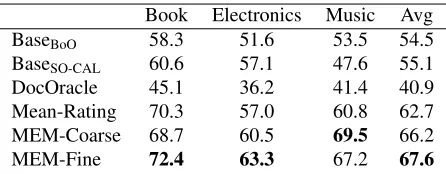
[image:9.612.309.550.60.107.2]5.3 Results for Strength Prediction
Book Electronics Music Avg
BaseBoO 58.3 51.6 53.5 54.5
BaseSO-CAL 60.6 57.1 47.6 55.1
DocOracle 45.1 36.2 41.4 40.9
Mean-Rating 70.3 57.0 60.8 62.7
MEM-Coarse 68.7 60.5 69.5 66.2
[image:10.612.74.297.56.143.2]MEM-Fine 72.4 63.3 67.2 67.6
Table 3: Accuracy of strength prediction.
6 Conclusion
We proposed the Multi-Experts Model for analyz-ing both opinion polarity and opinion strength at the sentence level. MEM is weakly supervised; it can run without any fine-grained annotations but is also able to leverage such annotations when avail-able. MEM is driven by a novel multi-expert prior, which integrates a number of diverse base predictors and propagates information across sentences using a sentiment-augmented word sequence kernel. Our ex-periments indicate that MEM achieves better overall accuracy than alternative methods.
References
Mikhail Belkin, Partha Niyogi, and Vikas Sindhwani. 2006. Manifold regularization: A geometric frame-work for learning from labeled and unlabeled examples.
The Journal of Machine Learning Research, 7:2399– 2434.
Christopher M. Bishop. 2006. Pattern recognition and machine learning, volume 4. Springer New York. Nicola Cancedda, ´Eric Gaussier, Cyril Goutte, and
Jean-Michel Renders. 2003. Word-sequence kernels. Jour-nal of Machine Learning Research, 3:1059–1082. Oliver Chapelle, Bernhard Sch¨olkopf, and Alexander Zien.
2006.Semi-Supervised Learning. MIT Press.
Yejin Choi and Claire Cardie. 2009. Adapting a polarity lexicon using integer linear programming for domain-specific sentiment classification. InProceedings of the Conference on Empirical Methods in Natural Language Processing, volume 2, pages 590–598.
Wei Chu and Zoubin Ghahramani. 2006. Gaussian pro-cesses for ordinal regression. Journal of Machine Learning Research, 6(1):1019.
Thomas G. Dietterichl. 2002. Ensemble learning. The Handbook of Brain Theory and Neural Networks, pages 405–408.
Xiaowen Ding, Bing Liu, and Philip S. Yu. 2008. A holistic lexicon-based approach to opinion mining. In
Proceedings of the International Conference on Web Search and Data Mining, pages 231–240.
Saso Dzeroski and Bernard Zenko. 2004. Is combining classifiers with stacking better than selecting the best one? Machine Learning, 54(3):255–273.
Jerome H. Friedman, Trevor Hastie, and Rob Tibshirani. 2008. Regularization paths for generalized linear mod-els via coordinate descent. Technical report.
Guohong Fu and Xin Wang. 2010. Chinese sentence-level sentiment classification based on fuzzy sets. In
Proceedings of the International Conference on Com-putational Linguistics, pages 312–319. Association for Computational Linguistics.
Andrew B. Goldberg and Xiaojun Zhu. 2006. Seeing stars when there aren’t many stars: Graph-based semi-supervised learning for sentiment categorization. In
HLT-NAACL 2006 Workshop on Textgraphs: Graph-based Algorithms for Natural Language Processing. Minqing Hu and Bing Liu. 2004. Mining and
summariz-ing customer reviews. In Proceedings of the ACM SIGKDD Conference on Knowledge Discovery and Data Mining, pages 168–177.
Lun-Wei Ku, I-Chien Liu, Chia-Ying Lee, Kuan hua Chen, and Hsin-Hsi Chen. 2008. Sentence-level opinion anal-ysis by copeopi in ntcir-7. InProceedings of NTCIR-7 Workshop Meeting.
Yi Mao and Guy Lebanon. 2006. Isotonic Conditional Random Fields and Local Sentiment Flow. Advances in Neural Information Processing Systems, pages 961– 968.
Ryan T. McDonald, Kerry Hannan, Tyler Neylon, Mike Wells, and Jeffrey C. Reynar. 2007. Structured models for fine-to-coarse sentiment analysis. InProceedings of the Annual Meeting on Association for Computational Linguistics, volume 45, page 432.
George A. Miller. 1995. WordNet: a lexical database for English. Communications of the ACM, 38(11):39–41.
Bo Pang and Lillian Lee. 2004. A sentimental education: Sentiment analysis using subjectivity summarization based on minimum cuts. InProceedings of the Annual Meeting on Association for Computational Linguistics, pages 271–278.
Bo Pang and Lillian Lee. 2005. Seeing stars: Exploiting class relationships for sentiment categorization with respect to rating scales. InProceedings of the Annual Meeting of the Association for Computational Linguis-tics, pages 124–131.
Guang Qiu, Bing Liu, Jiajun Bu, and Chun Chen. 2009. Expanding Domain Sentiment Lexicon through Dou-ble Propagation. InInternational Joint Conference on Artificial Intelligence, pages 1199–1204.
Lizhen Qu, Georgiana Ifrim, and Gerhard Weikum. 2010. The bag-of-opinions method for review rating predic-tion from sparse text patterns. InProceedings of the International Conference on Computational Linguis-tics, pages 913–921.
Carl Edward Rasmussen. 2004. Gaussian processes in machine learning. Springer.
Maite Taboada, Julian Brooke, Milan Tofiloski, Kim-berly D. Voll, and Manfred Stede. 2011. Lexicon-based methods for sentiment analysis. Computational Linguistics, 37(2):267–307.
Oscar T¨ackstr¨om and Ryan T. McDonald. 2011a. Dis-covering Fine-Grained Sentiment with Latent Variable Structured Prediction Models. InProceedings of the European Conference on Information Retrieval, pages 368–374.
Oscar T¨ackstr¨om and Ryan T. McDonald. 2011b. Semi-supervised latent variable models for sentence-level
sentiment analysis.In Proceedings of the Annual Meet-ing of the Association for Computational LMeet-inguistics, pages 569–574.
Theresa Wilson, Janyce Wiebe, and Paul Hoffmann. 2005. Recognizing contextual polarity in phrase-level senti-ment analysis. InProceedings of the Human Language Technology Conference and the Conference on Empir-ical Methods in Natural Language Processing, pages 347–354.
Xiaojin Zhu and Zoubin Ghahramani. 2002. Learning from labeled and unlabeled data with label propagation. Technical report.
Xiaojin Zhu, Zoubin Ghahramani, and John Lafferty. 2003. Semi-supervised learning using Gaussian fields and harmonic functions. InProceedings of the Inter-national Conference on Machine Learning, pages 912– 919.