Aggregate and mixed order Markov models for statistical language processing

(1)

Aggregate and m i x e d - o r d e r Markov models for

statistical language processing

L a w r e n c e S a u l a n d F e r n a n d o P e r e i r a

{Isaul, pereira}©research, att.

c o m

A T ~ T L a b s - R e s e a r c h 180 P a r k A v e , D - 1 3 0 F l o r h a m P a r k , N J 0 7 9 3 2

A b s t r a c t

We consider the use of language models whose size and accuracy are intermediate between different order n-gram models. Two types of models are studied in particular. Aggregate Markov models are class- based bigram models in which the mapping from words to classes is probabilistic. Mixed-order Markov models combine bigram models whose predictions are conditioned on different words. Both types of models are trained by Expectation- Maximization (EM) algorithms for maximum likelihood estimation. We examine smoothing procedures in which these models are interposed between different order n-grams. This is found to significantly reduce the perplexity of unseen word combinations.

1 I n t r o d u c t i o n

The purpose of a statistical language model is to assign high probabilities to likely word sequences and low probabilities to unlikely ones. The challenge here arises from the combinatorially large n u m b e r of possibilities, only a fraction of which can ever be observed. In general, language models must learn to recognize word sequences that are functionally similar but lexically distinct. The learning problem, one of generalizing from sparse data, is particularly acute for large-sized vocabularies (Jelinek, Mercer, and Roukos, 1992).

The simplest models of natural language are n- gram Markov models. In these models, the probability of each word depends on the n - 1 words that precede it. T h e problems in estimating ro- bust models of this form are well-documented. T h e number of p a r a m e t e r s - - o r transition probabilities-- scales as V n, where V is the vocabulary size. For typical models (e.g., n = 3, V = 104), this number exceeds by m a n y orders of magnitude the total number of words in any feasible training corpus.

T h e transition probabilities in n-gram models are estimated from the counts of word combinations in the training corpus. Maximum likelihood (ML) estimation leads to zero-valued probabilities for unseen n-grams. In practice, one adjusts or smoothes (Chen and G o o d m a n , 1996) the ML estimates so that the language model can generalize to new phrases. Smoothing can be done in many w a y s - - f o r example, by introducing artificial counts, backing off to lower- order models (Katz, 1987), or combining models by interpolation (Jelinek and Mercer, 1980).

Often a great deal of information:is lost in the smoothing procedure. This is due to the great dis- crepancy between n-gram models of different order. The goal of this paper is to investigate models that are intermediate, in both size and accuracy, between different order n-gram models. We show that such models can "intervene" between different order n- grams in the smoothing procedure. Experimentally, we find that this significantly reduces the perplexity of unseen word combinations.

T h e language models in this paper were evalu- ated on the ARPA North American Business News (NAB) corpus. All our experiments used a vocabulary of sixty-thousand words, including tokens for punctuation, sentence boundaries, and an unknown word token standing for all out-of-vocabulary words. T h e training d a t a consisted of approxi- mately 78 million words (three million sentences); the test data, 13 million words (one-half million sentences). All sentences were drawn randomly without replacement from the NAB corpus. All perplexity figures given in the paper are computed by combining sentence probabilities; the probability of sentence wow1 . . . w ~ w n + l is given by

yIn+lP(wilwo ..wi-1),

_{i = 1} where w0 and wn+l are the start- and end-of-sentence markers, respectively. Though not reported below, we also confirmed that the results did not vary significantly for different randomly drawn test sets of the same size.

T h e organization of this paper is as follows. In Section 2, we examine aggregate Markov models, or class-based bigram models (Brown et al., 1992) in which the mapping from words to classes

(2)

is probabilistic. We describe an iterative algorithm for discovering "soft" word classes, based on the Expectation-Maximization (EM) procedure for maximum likelihood estimation (Dempster, Laird, and Rubin, 1977). Several features make this algorithm attractive for large-vocabulary language modeling: it has no tuning parameters, converges monotonically in the log-likelihood, and handles probabilistic constraints in a natural way. The number of classes, C, can be small or large depending on the constraints of the modeler. Varying the number of classes leads to models that are intermediate between unigram (C = 1) and bigram (C = V) models.

In Section 3, we examine another sort of "intermediate" model, one t h a t arises from combinations of non-adjacent words. Language models using such combinations have been proposed by Huang

et al.

(1993), Ney, Essen, and Kneser (1994), and Rosen- feld (1996), among others. We consider specifically the

skip-k

transition matrices,

M(wt_k, wt),

whose predictions are conditioned on the kth previous word in the sentence. (The value of k determines how many words one "skips" back to make the prediction.) These predictions, conditioned on only a single previous word in the sentence, are inherently weaker than those conditioned on all k previous words. Nevertheless, by combining several predictions of this form (for different values of k), we can create a model t h a t is intermediate in size and accuracy between bigram and trigram models.

Mixed-order

Markov models express the predictions

P(wt[wt-1, wt-2,..., Wt-m)

as a convex combination of skip-k transition matrices,

M(wt-k, wt).

We derive an EM algorithm to learn the mixing coefficients, as well as the elements of the transition matrices. The number of transition probabilities in these models scales as

mV 2, as

opposed to V m+l. Mixed-order models are not as powerful as trigram models, but they can make much stronger predictions than bigram models. T h e reason is that quite often the immediately preceding word has less predictive value than earlier words in the same sentence.

In Section 4, we use aggregate and mixed-order models to improve the probability estimates from n-grams. This is done by interposing these models between different order n-grams in the smoothing procedure. We compare our results to a baseline trigram model that backs off to bigram and unigram models. The use of "intermediate" models is found to reduce the perplexity of unseen word combinations by over 50%.

In Section 5, we discuss some extensions to these models and some open problems for future research. We conclude that aggregate and mixed-order models provide a compelling alternative to language models based exclusively on n-grams.

2 A g g r e g a t e M a r k o v m o d e l s

In this section we consider how to construct class- based bigram models (Brown

et al.,

1992). T h e problem is naturally formulated as one of hidden variable density estimation. Let

P(clwl )

denote the probability that word wl is m a p p e d into class c. Likewise, let

P(w21c)

denote the probability that words in class c are followed by the word w2. T h e class-based bigram model predicts t h a t word wl is followed by word w2 with probability

c

P(w21wl) = Z P(w21c)P(clwx)'

(1) c = l

where C is the total number of classes. T h e hidden variable in this problem is the class label c, which is unknown for each word wl. Note t h a t eq. (1) represents the V 2 elements of the transition m a t r i x

P(w21wa)

in terms of the

2CV

elements of

P(w2]c)

and

P(clwl ).

T h e Expectation-Maximization (EM) algorithm (Dempster, Laird, and Rubin, 1977) is an iterative procedure for estimating the parameters of hidden variable models. Each iteration consists of two steps: an E-step which computes statistics over the hidden variables, and an M-step which updates the parameters to reflect these statistics.

T h e EM algorithm for aggregate Markov models is particularly simple. The E-step is to compute, for each bigram

WlW 2

in the training set, the

posterior

probability

P(w2]c)P(C[Wl)

(2)

P(ClWl, w2) = ~c, P(w2lc')P(c'lwl)"

Eq. (2) gives the probability that word wl was assigned to class

c,

based on the observation that it was followed by word w2. T h e M-step uses these posterior probabilities to re-estimate the model parameters. T h e updates for aggregate Markov models are:

~ w N(wl, w)P(ClWl, w)

P(clwl) ~

~wc, N(wl

_,

_{w)P(c [wl,}

'

_{w )}

,

₍₃₎

Ew N(w, w2)P(clw, w~)

P(w2[c) ~- Eww'g(w,w')P(clw, w')'

(4)

where N(Wl, w2) denotes the number of counts of

wlw2

in the training set. These updates are guar- anteed to increase the overall log-likelihood,

g= Z

N(Wl'W2)lnP(w21wl)'

(5) W l W 2

at each iteration. In general, they converge to a local (though not global) m a x i m u m of the log-likelihood. T h e perplexity V* is related to the log-likelihood by

V*

: e - ~ / N , where N is the total n u m b e r of words processed.

(3)

100( 9o( 80(

4O(

20(

1000 goo 80~

41111

2@

5 10 15 20 25 30 5 10 15 20 25 30

iteration of EM iteration of EM

(a)

(b)

Figure 1: Plots of (a) training and (b) test perplexity versus number of iterations of the EM algorithm, for the aggregate Markov model with C = 32 classes.

C train test 1 964.7 964.9 2 771.2 772.2 4 541.9 543.6 8 399.5 401.5 16 328.8 331.8 32 278.9 283.2 V 123.6 - -

Table 1: Perplexities of aggregate Markov models on the training and test sets; C is the number of classes. T h e case C = 1 corresponds to a ML unigram model; C = V, to a ML bigram model.

0.2 0.4 0.6 0.8

winning assignment probability

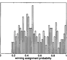
Figure 2: Histogram of the winning assignment probabilities, maxc

P(clw),

for the three hundred most commonly occurring words.

for performing the decomposition in eq. (1), it is worth noting t h a t only the EM algorithm directly optimizes the log-likelihood in eq. (5). This has ob- vious advantages if the goal of finding word classes is to improve the perplexity of a language model. The EM algorithm also handles probabilistic constraints in a natural way, allowing words to belong to more than one class if this increases the overall likelihood. Our approach differs in important ways from the use of hidden Markov models (HMMs) for class- based language modeling (Jelinek

et al.,

1992). While HMMs also use hidden variables to represent word classes, the dynamics are fundamentally different. In HMMs, the hidden state at time t ÷ 1 is predicted (via the state transition matrix) from the hidden state at time t. On the other hand, in aggregate Markov models, the hidden state at time t + 1 is predicted (via the matrix

P(ct+llwt))

from the

word

at time t. T h e state-to-state versus word-to- state dynamics lead to different learning algorithms. For example, the Baum-Welch algorithm for HMMs requires forward and backward passes through each training sentence, while the EM algorithm we use does not.

We trained aggregate Markov models with 2, 4, 8, 16, and 32 classes. Figure 1 shows typical plots of the training and test set perplexities versus the number of iterations of the EM algorithm. Clearly, the two curves are very close, and the monotonic decrease in test set perplexity strongly suggests lit- tle if any overfitting, at least when the number of classes is small compared to the number of words in the vocabulary. Table 1 shows the final perplexities (after thirty-two iterations of EM) for various aggregate Markov models. These results confirm that aggregate Markov models are intermediate in accuracy between unigram (C = 1) and bigram (C = V) models.

T h e aggregate Markov models were also observed to discover meaningful word classes. Table 2 shows, for the aggregate model with C = 32 classes, the

[image:3.612.144.466.74.203.2] [image:3.612.136.228.290.384.2] [image:3.612.110.252.508.636.2]

(4)

las

cents made make take

ago day earfier Friday Monday month quarter reported said Thursday trading Tuesday Wednesday ( . . . )

even get to

based days down home months up work years

those (,) (--)

(.) (?)

eighty fifty forty ninety seventy sixty thirty

19 bilfion hundred million nineteen

20 did (") (')

21 but called San (:) (start-of-sentence)

22

23

bank board chairman end group members number office out part percent price prices rate sales shares use

a an another any dollar each first good her his its my old our their this

24 long Mr. year

7

twenty (0 (') 25

8 can could may should to will would 9 about at just only or than (&) (;)

i

10 economic high interest much no such tax united i 27 well

11 president

12 because do how if most say so then think very

what when where 29

13 according back expected going him plan used way 15 don't I people they we you [

Bush company court department more officials ] 30 16

pofice retort spokesman [

17 former the

American big city federal general house mifitary 18 national party political state union York i

business California case companies corporation dollars incorporated industry law money thousand time today war week 0) (unknown) 26 also government he it market she that there

which who

A. B. C. D. E. F. G. I. L. M. N. P. R. S. T. U. 28 both foreign international major many new oil

other some Soviet stock these west world

after all among and before between by during for from in including into like of off on over since through told under until while with

eight fifteen five four half last next nine oh one second seven several six ten third three twelve two zero (-)

31 are be been being had has have is it's not still was were

32 chief exchange news public service trade

Table 2: Most probable assignments for the 300 most frequent words in an aggregate Markov model with C = 32 classes. Class 14 is absent because it is not the most probable class for any of the selected words.)

most probable class assignments of the three hundred most c o m m o n l y occurring words. To be precise, for each class c*, we have listed the words for which c* = arg maxe

P(c]w).

Figure 2 shows a histogram of the winning assignment probabilities, maxe

P(c[w),

for these words. Note t h a t the winning assignment probabilities are distributed broadly over the inter- val [-~, 1]. This demonstrates the utility of allowing "soft" membership classes: for most words, the max- i m u m likelihood estimates of

P(clw )

do not corre- spond to a winner-take-all assignment, and therefore any method that assigns each word to a single class ("hard" clustering), such as those used by Brown

et

al.

(1992) or Ney, Essen, and Kneser (1994), would lose information.

We conclude this section with some final com- ments on overfitting. Our models were trained by thirty-two iterations of EM, allowing for nearly com- plete convergence in the log-likelihood. Moreover, we did not implement any flooring constraints 1 on the probabilities

P(clwl )

or

P(w21c).

Nevertheless, in all our experiments, the ML aggregate Markov

lit is worth noting, in this regard, that individual zeros in the matrices

P(w2[c)

and

P(c[wl)

do not nec- essarily give rise to zeros in the matrix

P(w21wt),

as computed from eq. (1).

models assigned non-zero probability to all the bigrams in the test set. This suggests t h a t for large vocabularies there is a useful regime 1 << C << V in which aggregate models do not suffer much from overfitting. In this regime, aggregate models can be relied upon to compute the probabilities of unseen word combinations. We will return to this point in Section 4, when we consider how to s m o o t h n - g r a m language models.

3 M i x e d - o r d e r M a r k o v m o d e l s

One of the drawbacks of n-gram models is t h a t their size grows rapidly with their order. In this section, we consider how to make predictions based on a convex combination of'pairwise correlations. This leads to language models whose size grows

linearly

in the number of words used for each prediction.

For each k > 0, the

ski_p-k

transition m a t r i x

M(wt-k, wt)

predicts the current word from the

kth previous word in the sentence. A

mixed-order

Markov model combines the information in these matrices for different values of k. Let m denote the number of bigram models being combined. The probability distribution for these models has the form:

[image:4.612.89.543.81.371.2]

(5)

k - 1

f i Ak(wt-k)

Mk(wt-k,Wt)

II[1-

Aj(w,_~)].

k = l j = l

T h e t e r m s in this equation have a simple interpreta- tion. T h e V x V matrices Mk (w, w') in eq. (6) de- fine the skip-k stochastic dependency of w' at some position t on w at position t - k; the p a r a m e t e r s Ak (w) are mixing coefficients t h a t weight the predictions f r o m these different dependencies. T h e value of Ak (w) can be interpreted as the probability t h a t the model, upon seeing the word wt-k, looks no further back to m a k e its prediction (Singer, 1996). T h u s the model predicts from wt-1 with probability A1

(wt-1),

f r o m w t - 2 with probability [1 -

Al(wt-1)]A2(wt-~),

and so on. T h o u g h included in eq. (6) for cosmetic reasons, the p a r a m e t e r s Am (w) are actually fixed to unity so t h a t the model never looks further t h a n m words back.

We can view eq. (6) as a hidden variable model. I m a g i n e t h a t we adopt the following s t r a t e g y to predict the word at t i m e t. Starting with the previous word, we toss a coin (with bias

Ai(Wt_i) ) to

see if this word has high predictive value. If the answer is yes, then we predict from the skip-1 transition m a t r i x ,

Ml(Wt-l,Wt).

Otherwise, we shift our at- tention one word t o t h e left and repeat the process. If after m - 1 tosses we have not settled on a prediction, then as a last resort, we make a prediction using

Mm(wt-m, wt).

T h e hidden variables in this process are the outcomes of the coin tosses, which are unknown for each word

wt-k.

Viewing the model in this way, we can derive an EM algorithm to learn the mixing coefficients Ak (w) and the transition matrices 2

Mk(w, w').

T h e E-step of the algorithm is to compute, for each word in the training set, the posterior probability t h a t it was generated by

Mk(wt-k, wt).

Denoting these posterior probabilities by Ck(t), we have:

Ck(t) =

(7)

Aa(wt-a)Mk(wt-k wt) k-1

,

P(wt Iw,-1, w,-2,..., w,_~)

where the d e n o m i n a t o r is given by eq. (6). T h e M-step of the algorithm is to u p d a t e the p a r a m e - ters Ak(W) and

Mk(w, w')

to reflect the statistics in eq. (7). T h e u p d a t e s for mixed-order Markov models are given by:

,s(w, wt-k)¢k (0

A (w)

(8)

~Note that the ML estimates of

Mk(w,w')

do not depend only on the raw counts of k-separated bigrams; they are also coupled to the values of the mixing coefficients, Aa(w). In particular, the EM algorithm adapts the matrix elements to the weighting of word combinations in eq. (6). The raw counts of k-separated bigrams, however, do give good initial estimates.

11C

105

10~

"~ 95

85

8G

75

7G

1 2 3 4

iteration of E M

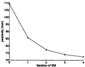
Figure 3: Plot of (training set) perplexity versus n u m b e r of iterations of the EM algorithm. T h e results are for the m = 4 mixed-order Markov model.

m train missing 1 123.2 0.045 2 89.4 0.014 3 77.9 0.0063 4 72.4 0.0037

Table 3: Results for ML mixed-order models; m denotes the n u m b e r of b i g r a m s t h a t were mixed into each prediction. T h e first column shows the perplexities on the training s e t . T h e s.ec0nd shows the fraction of words in the test set t h a t were assigned zero probability. T h e case m = 1 corresponds to a ML bigram model.

Mk(w, W') +- ~ t ~(W, Wt-k)~(W',

Wt)¢k(t)

E ,

w,-k)¢k(t)

, (9)

where the sums are over all the sentences in the training set, and J(w, w') = 1 iff w = w'.

We trained mixed-order Markov models with 2 < m _< 4. Figure 3 shows a typical plot of the training set perplexity as a function of the n u m b e r of iterations of the EM algorithm. Table 3 shows the final perplexities on the training set (after four iterations of EM). Mixed-order models cannot be used directly on the test set because they predict zero probability for unseen word combinations. Unlike standard n - g r a m models, however, the n u m b e r of unseen word combinations actually

decreases

with the order of the model. T h e reason for this is t h a t mixed-order models assign finite probability to all n- grams

wlw~ ... wn

for which

any

of the k-separated bigrams

wkwn

are observed in the training set. To illustrate this point, Table 3 shows the fraction of words in the test set t h a t were assigned zero probability by the mixed-order model. As expected, this fraction decreases monotonically with the n u m b e r of bigrams t h a t are mixed into each prediction.

Clearly, the success of mixed-order models depends on the ability to gauge the predictive value of each word, relative to earlier words in the same sentence. Let us see how this plays out for the

[image:5.612.354.499.69.183.2] [image:5.612.370.477.242.301.2]

(6)

0.1 < A l ( w ) < 0.7

(-) and of (") or (;) to (,) (&) by with S. from nine were for that eight low seven the (() (:) six are not against was four between a their two three its (unknown) S. on as is (--) five 0) into C. M. her him over than A.

0.96 < Al(w) < 1

officials prices which go way he last they earlier an Tuesday there foreign quarter she former federal don't days Friday next Wednesday (%) Thursday I Monday Mr. we half based part United it's years going nineteen thousand months (.) million very cents San ago U. percent billion (?) according (.)

Table 4: Words with low and high values of Al(w) in an m = 2 mixed order model.

second-order (m = 2) model in Table 3. In this model, a small value for ~l(w) indicates that the word w typically carries less information that the word that precedes it. On the other hand, a large value for Al(w) indicates that the word w is highly predictive. The ability to learn these relationships is confirmed by the results in Table 4. Of the three- hundred most c o m m o n words, Table 4 shows the fifty with the lowest and highest values of Al(w). Note how low values of Al(w) are associated with prepositions, mid-sentence punctuation marks, and conjunctions, while high values are associated with "contentful" words and end-of-sentence markers. (A particularly interesting dichotomy arises for the two forms "a" and "an" of the indefinite article; the lat- ter, because it always precedes a word that begins with a vowel, is inherently more predictive.) These results underscore the importance of allowing the coefficients Al(w) to depend on the context w, as opposed to being context-independent (Ney, Essen, and Kneser, 1994).

4 S m o o t h i n g

Smoothing plays an essential role in language models where ML predictions are unreliable for rare events. In n-gram modeling, it is c o m m o n to adopt a recursive strategy, smoothing bigrams by unigrams, trigrams by bigrams, and so on. Here we adopt a similar strategy, using the (m - 1)th mixed-order model to smooth the ruth one. At the "root" of our smoothing procedure, however, lies not a unigram model, but an aggregate Markov model with C > 1 classes. As shown in Section 2, these models assign finite probability to all word combinations, even those that are not observed in the training set. Hence, they can legitimately replace unigrams as the base model in the smoothing procedure.

Let us first examine the impact of replacing unigram models by aggregate models at the root of the

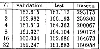
C 1 2 4 8 16 32

validation test unseen 163.615

162.982 161.513 161.327 160.034 159.247

167.112 166.193 164.363 164.104 162.686 161.683

293175 259360 200067 190178 164673 150958

Table 5: Perplexities of bigram models smoothed by aggregate Markov models with different numbers of classes (C).

smoothing procedure. To this end, a held-out interpolation algorithm (Jelinek and Mercer, 1980) was used to smooth an ML bigram model with the aggregate Markov models from Section 2. T h e smoothing parameters, one for each row of the bigram transition matrix, were estimated from a validation set the same size as the test set. Table 5 gives the final perplexities on the validation set, the test set, and the unseen bigrams in the test set. Note t h a t smoothing with the C = 32 aggregate Markov model has nearly halved the perplexity of unseen bigrams, as compared to smoothing with the unigram model.

Let us now examine the recursive use of mixed- order models to obtain smoothed probability estimates. Again, a held-out interpolation algorithm was used to smooth the mixed-order Markov models from Section 3. The ruth mixed-order model had

m V smoothing parameters 0"k (w), corresponding to

the V rows in each skip-k transition matrix. T h e m t h mixed-order model was smoothed by discount- ing the weight of each skip-k prediction, then fill- ing in the leftover probability mass by a lower-order model. In particular, the discounted weight of the skip-k prediction was given by

k - 1

[1 - O ' k ( w t - k ) l A k ( W t - k ) H I 1 --)~j(wt-j)] , (10)

j = l

leaving a total mass of

k - 1

fi O'k(Wt-k)~k(W,-k)

H[1--

,~j(W,_j)]

(11)

k = l j = l

for the ( m - 1)th mixed-order model. (Note that the m = 1 mixed-order model corresponds to a ML bigram model.)

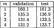
[image:6.612.84.304.69.222.2] [image:6.612.355.520.73.154.2]

(7)

m validation test 1 160.1 161.3 2 135.3 136.9 3 131.4 133.5 4 131.2 133.7

Table 6: Perplexities of s m o o t h e d mixed-order m o d - els on the validation and test sets.

to an m = 3 mixed-order model, s m o o t h e d by a m = 2 mixed-order model, s m o o t h e d by a ML bi- g r a m model, etc. A significant decrease in perplexity occurs in moving to the s m o o t h e d m = 2 mixed- order model. On the other hand, the difference in perplexity for higher values of m is not very dra- matic.

Our last experiment looked at the smoothing of a t r i g r a m model. Our baseline was a ML t r i g r a m model t h a t backed off 3 to b i g r a m s (and when nec- essary, unigrams) using the K a t z backoff procedure (Katz, 1987). In this procedure, the predictions of the ML t r i g r a m model are discounted by an a m o u n t determined by the G o o d - T u r i n g coefficients; the leftover probability mass is then filled in by the backoff model. We c o m p a r e d this to a t r i g r a m model t h a t backed off to the m = 2 model in Table 6. This was handled by a slight variant of the K a t z procedure (Dagan, Pereira, and Lee, 1994) in which the mixed- order model substituted for the backoff model.

One advantage of this smoothing procedure is t h a t it is straightforward to assess the performance of different backoff models. Because the backoff models are only consulted for unseen word combinations, the perplexity on these word combinations serves as a reasonable figure-of-merit.

Table 7 shows those perplexities for the two smoothed t r i g r a m models (baseline and backoff). T h e mixed-order s m o o t h i n g was found to reduce the perplexity of unseen word combinations by 51%. Also shown in the table are the perplexities on the entire test set. T h e overall perplexity decreased by 1 6 % - - a significant a m o u n t considering t h a t only 24% of the predictions involved unseen word combinations and required backing off from the t r i g r a m model.

T h e models in Table 7 were constructed from all n - g r a m s (1 < n < 3) observed in the training data. Because m a n y n - g r a m s occur very infrequently, a natural question is whether truncated models, which o m i t low-frequency n - g r a m s f r o m the training set, can perform as well as untruncated ones. T h e advantage of truncated models is t h a t they do not need to store nearly as m a n y non-zero p a r a m e t e r s as untruncated models. T h e results in Table 8 were ob- ~We used a backoff procedure (instead of interpolation) to avoid the estimation of trigram smoothing parameters.

backoff test unseen baseline 95.2 2799

mixed 79.8 1363

Table 7: Perplexities of two s m o o t h e d t r i g r a m m o d - els on the test set and the subset of unseen word combinations. T h e baseline model backed off to bi- g r a m s and unigrams; the other backed off to the m = 2 model in Table 6.

t baseline mixed t r i g r a m s ( × 105) missing

1 95.2 79.8 25.4 0.24

2 98.6 78.3 6.1 0.32

3 101.7 79.6 3.3 0.36

4 104.2 81.1 2.3 0.38

5 106.2 82.4 1.7 0.41

Table 8: Effect of truncating t r i g r a m s t h a t occur less t h a n t times. T h e table shows the baseline and mixed-order perplexities on the test set, the number of distinct trigrams with t or more counts, and the fraction of trigrams in the test set t h a t required backing off.

tained by dropping trigrams t h a t occurred less t h a n t times in the training corpus. T h e t = 1 row corresponds to the models in Table 7. T h e m o s t interesting observation from the table is t h a t o m i t t i n g very low-frequency trigrams does not decrease the quality of the mixed-order model, and m a y in fact slightly improve it. This contrasts with the s t a n d a r d backoff model, in which truncation causes significant increases in perplexity.

5 D i s c u s s i o n

Our results d e m o n s t r a t e the utility of language models t h a t are intermediate in size and accuracy between different order n - g r a m models. T h e two models considered in this paper were hidden variable Markov models trained by EM algorithms for m a x i m u m likelihood estimation. C o m b i n a t i o n s of intermediate-order models were also investigated by Rosenfeld (1996). His experiments used the 20,000- word vocabulary Wall Street Journal corpus, a pre- decessor of the NAB corpus. He trained a m a x i m u m - entropy model consisting of unigrams, bigrams, trigrams, skip-2 bigrams and trigrams; after selecting long-distance b i g r a m s (word triggers) on 38 million words, the model was tested on a held-out 325 thousand word sample. Rosenfeld reported a test-set perplexity of 86, a 19% reduction from the 105 perplexity of a baseline t r i g r a m backoff model. In our experiments, the perplexity gain of the mixed-order model ranged from 16% to 22%, depending on the a m o u n t of truncation in the t r i g r a m model.

While Rosenfeld's results and ours are not di-

[image:7.612.128.240.73.131.2] [image:7.612.368.484.74.109.2] [image:7.612.314.544.189.260.2]

(8)

rectly comparable, both demonstrate the utility of mixed-order models. It is worth discussing, however, the different approaches to combining information from non-adjacent words. Unlike the maximum entropy approach, which allows one to combine m a n y non-independent features, ours calls for a careful Markovian decomposition. Rosenfeld ar- gues at length against naive linear combinations in favor of m a x i m u m entropy methods. His arguments do not apply to our work for several reasons. First, we use a large number of context-dependent mixing parameters to optimize the overall likelihood of the combined model. Thus, the weighting in eq. (6) en- sures that the skip-k predictions are only invoked when the context is appropriate. Second, we adjust the predictions of the skip-k transition matrices (by EM) so that they match the contexts in which they are invoked. Hence, the count-based models are interpolated in a way that is "consistent" with their eventual use.

Training efficiency is another issue in evaluating language models. The m a x i m u m entropy m e t h o d requires very long training times: e.g., 200 CPU- days in Rosenfeld's experiments. Our methods re- quire significantly less; for example, we trained the smoothed m = 2 mixed-order model, from start to finish, in less than 12 CPU-hours (while using a larger training corpus). Even accounting for differ- ences in processor speed, this amounts to a significant mismatch in overall training time.

In conclusion, let us mention some open problems for further research. Aggregate Markov models can be viewed as approximating the full bigram transition m a t r i x by a m a t r i x of lower rank. (From eq. (1), it should be clear that the rank of the class- based transition m a t r i x is bounded by the number of classes, C.) As such, there are interesting parallels between Expectation-Maximization (EM), which minimizes the approximation error as measured by the KL divergence, and singular value decomposition (SVD), which minimizes the approximation error as measured by the L2 norm (Press

et al., 1988; Schiitze, 1992). Whereas SVD finds a

global m i n i m u m in its error measure, however, EM only finds a local one. It would clearly be desirable to improve our understanding of this fundamental problem.

In this paper we have focused on bigram models, but the ideas and algorithms generalize in a straightforward way to higher-order n-grams. Aggregate models based on higher-order n-grams (Brown et al.,

1992) might be able to capture multi-word struc- tures such as noun phrases. Likewise, trigram-based mixed-order models would be useful complements to 4-gram and 5-gram models, which are not uncom- mon in large-vocabulary language modeling.

A final issue that needs to be addressed is s c a l i n g - - t h a t is, how the performance of these models depends on the vocabulary size and a m o u n t

of training data. Generally, one expects that the sparser the data, the more helpful are models t h a t can intervene between different order n-grams. Nev- ertheless, it would be interesting to see exactly how this relationship plays out for aggregate and mixed- order Markov models.

Acknowledgments

We thank Michael Kearns and Yoram Singer for useful discussions, the anonymous reviewers for ques- tions and suggestions that helped improve the paper, and Don Hindle for help with his language modeling tools, which we used to build the baseline models considered in the paper.

References

P. Brown, V. Della Pietra, P. deSouza, J. Lai, and R. Mercer. 1992. Class-based n-gram models of natural language. Computational Linguistics 18(4):467-479.

S. Chen and J. G o o d m a n . 1996. An empirical study of smoothing techniques for language modeling. In

Proceedings of the 34th Meeting of the Association for Computational Linguistics.

I. Dagan, F. Pereira, and L. Lee. 1994. Similarity- based estimation of word co-occurrence probabilities. In Proceedings of the 32nd Annual Meeting of the Association for Computational Linguistics.

A. Dempster, N. Laird, and D. Rubin. 1977. Max- imum likelihood from incomplete d a t a via the EM algorithm. Journal of the Royal Statistical Society

B39:1-38.

X. Huang, F. Alleva, H. Hon, M.-Y. Hwang, K.-F. Lee, and R. Rosenfeld. 1993. T h e S P H I N X - I f speech

recognition system: an overview. Computer Speech

and Language, 2:137-148.

F. Jelinek and R. Mercer. 1980. Interpolated estimation of Markov source parameters from sparse data. In Proceedings of the Workshop on Pattern Recognition in Practice.

F. Jelinek, R. Mercer, and S. Roukos. 1992. Princi- ples of lexical language modeling for speech recognition. In S. Furui and M. Sondhi, eds. Advances in

Speech Signal Processing. Mercer Dekker, Inc.

S. Katz. 1987. Estimation of probabilities from sparse d a t a for the language model component of a speech recognizer. IEEE Transactions on ASSP

35(3):400-401.

(9)

F. Pereira, N. Tishby, and L. Lee. 1993. Distribu-

tional clustering of English words. In Proceedings

of the 30th Annual Meeting of the Association for Computational Linguistics.

W. Press, B. Flannery, S. Teukolsky, and W. Vet-

terling. 1988. Numerical Recipes in C. Cambridge

University Press: Cambridge.

R. Rosenfeld. 1996. A Maximum Entropy Approach

to Adaptive Statistical Language Modeling. Com-