Energy, Environment, and Economy Interactions in Iran with Cointegrated and ECM Simultaneous Model

Munich Personal RePEc Archive

Energy, Environment, and Economy

Interactions in Iran with Cointegrated

and ECM Simultaneous Model

Mohamad Taghvaee, Vahid and Seifi Aloo, Alireza and

Khodaparast Shirazi, Jalil

Persian Gulf University, Azad University of Mazandaran, Azad

University of Shiraz

2016

Online at

https://mpra.ub.uni-muenchen.de/70508/

1

Procedia of Economics and Finance

Energy, Environment, and Economy Interactions in Iran with

Cointegrated and ECM Simultaneous Model

Vahid Mohamad Taghavee

_{, Alireza Seifi Aloo}

_{, Jalil Khodaparast Shirazi}

a_{Persian Gulf University, Bushehr,Iran} b_{Mazandaran University, Babolsar, Iran}

c_{Azad University of Shiraz, Shiraz, Iran}

Abstract

Nobody on the planet is going to be untouched by the impacts of climate change. This study aims to arrange the various socioeconomic elasticities of environmental pollution in order of priority, depending on the length of time period, to establish the most effective policy. We employed a simultaneous equations system to find out the various socioeconomic elasticities in the long run and short run in Iran during 1974-2012. Based on the results, per capita CO2 emissions, GDP, energy consumption show the strongest interactions (relationships and elasticities) in the equations system as a whole in the long run. Moreover, it is the trade openness, labour force, financial development, and urbanization which show the most decisive effects in the short run. So the effectiveness of the system variables depends on the time period. Trade openness, labour force, and financial development play the most leading role in the short run, notwithstanding their limited role in the long run. However, energy consumption elasticity of CO2 emissions and urbanization elasticity of energy consumption are among the largest elasticities both in short run and long run. Therefore, energy consumption, economic growth and urbanization should be reduced and financial sector should be grown to decrease the environmental pollution. Moreover, economic growth is an effective factor for the long run; and trade openness and financial development are effective for the short run but urbanization and energy consumption are influential for both the long run and short run policies.

Keywords:Energy Consumption; Environmental Pollution; Economic Growth

1.Introduction

“Nobody on the planet is going to be untouched by the impacts of climate change” said the chairman of the Intergovernmental Panel on Climate Change in Japan, in 2014. The scientific proofs’ level of climate change effects has doubled since 2007. Climate change poses serious threat of severe shortage of food and water to the people who are breathing the polluted air. Moreover, the ocean acidification has increased dramatically. Not only are many species under the threat of extinction but also many have died out and vanished. Finally, which is important to the economists, each unit of temperature increment leads to loss in global income ranging from one tenth to one percent. Thus, the most polluting economies should be studied to stop back the climate change effects (IPCC Report, 2014; Taghvaee and Hajiani, 2015).

Iran is a good candidate for the environmental-economical studies owing to its polluting and energy-consuming economy. This country has only 0.005 percent share in global production while it has more than 0.15 percent share in global CO2 emissions, 30 times pollutant than productive (World Development Indicator). Despite the fact that economic growth may reduce environmental pollution in the higher level of income (Grossman and Kruger, 1991; Baek, 2015; Ge et al., 2015; Hao et al., 2015; Lee and Oh 2015; Taghvaee and Shirazi, 2014), Iran has not reached the high enough level (Taghvaee and Parsa, 2015); and it is within the range in which the more income, the more energy consumption and environmental pollution (Al-mulali, 2015; Taghvaee and Hajiani, 2014). Moreover, based on the climate and energy ranking of the Yale University, Iran is the hundredth country out of 178 which perform well. This rank is 128 for biodiversity and habitat, 117 for water sources, and 104 for health impacts. Therefore, Iran

Elsevier

2

should develop the cleaner sectors of the economy since its contribution in environmental pollution is 30 times greater than its contribution in global production (Taghvaee and Parsa, 2015) and it has one of the most pollutant economies among the other countries around the world.

There is a general consensus among the researchers on the environmental impacts of the various socioeconomic variables (such as economic growth, energy consumption, trade openness, financial development, urbanization, capital, and labour force) but the question is which one produces the greatest effect (Lotfalipour et al., 2010; Omri, 2013; Omri, 2014; Omri et al., 2015 Ren et al., 2014;. The policymakers should accurately evaluate the elasticity and effectiveness degree of each variable for adopting the most effective policies. Not only does the elasticity or effectiveness degree might vary from one variable to another variable but also the elasticity or effectiveness of each variable can fluctuate depending on the length of time period. Thus, the governors are advised to approve the strategically environmental plans for the most effective sectors depending on the length of time period and the level of management resulting in a long and dynamic chain of conscious decision making.

The main purpose of this study is to arrange the various socioeconomic elasticities of environmental pollution in order of priority, depending on the length of time period, to establish the most effective policy. The socioeconomic variables of the study include economic growth, energy consumption, trade openness, financial development, urbanization, capital, and labour force; and the time periods are short run and long run. The algorithm of the article is as follows: section 2 outlines the econometric modeling approach and describes the data used; section 3 depicts the empirical findings and finally section 4 holds the concluding annotations and offers some policy implications

2.Methodology and Data

Following Omri, 2013; Omri, 2014; Omri et al., 2015, we employed a simultaneous equations system to find out the various socioeconomic elasticities in the long run in Iran during 1974-2012. There are three equations in which carbon dioxide emissions, GDP, and energy consumption are the endogenous variables. The three-equation system is as follows:

(1)

= + + + + + +

(2)

= + + + + + + + +

(3)

= + + + + + + + +

where CO is the carbon dioxide emissions (per capita metric ton), GDP is per capita gross domestic production (constant Iranian Rial prices in 2004), E is energy consumption (per capita Kilogram oil equivalent), OP is trade openness (trade volume as a percentage of GDP), FD is financial development (domestic credit to private sector as a percentage of GDP), DR (is zero for the years before the Islamic revolution in 1979 and is one for the rest of the years) and DW (is one for the war years within 1980-1987 and is zero for the rest of the years) are dummy variables, LAB is the labour force (active population as a percentage of the total population), CAP is capital (per capita constant Iranian Rial prices in 2004), U is urban population (urban population as a percentage of the total population), is the residuals, t is the year, and L is the natural logarithm (meaning that all the variables are in the form of natural logarithm). Since the variables are in the natural logarithmic form, the parameters can be considered as the elasticities. All the variables derived from World Development Indicator other than per capita GDP, labour force, and capital which are come from the Central Bank of Islamic Republic of Iran.

Before the estimation of the system with 3SLS method, the variables are tested for stationarity and the system is tested for identification and exogeneity. We employed two unit root tests: Augmented Dickey Fuller (Dickey and Fuller, 1979) and Pillips Perron (Phillips and Perron, 1988). Both the tests are implemented in three cases: intercept, intercept and trend, and none of them. Then the variables with identical integration degree are tested for cointegration by Engle and Granger and Augmented Engle and Granger cointegration tests. According to the Engle and Granger and Augmented Engle and Granger methodology, the residuals of cointegrated equation must be stationary in level (Engle and Granger, 1987). After the variables’ tests, the system is tested for identification. A system is identified which has two rank and order conditions. Finally the exogeneity test is run to clarify if the exogenous variables are really exogenous (Gujarati, 2004).

3

(4)

= + + + + + + ̂ +

(5)

= + + + + + + +

+ ̂ +

(6)

= + + + + + + + + ̂

+

where d is one degree differentiation, ̂ _{is the estimated residuals in the cointegrated regression, e is the residual}

term, is the short run elasticity, and the remaining indices are as mentioned before.

3.Results

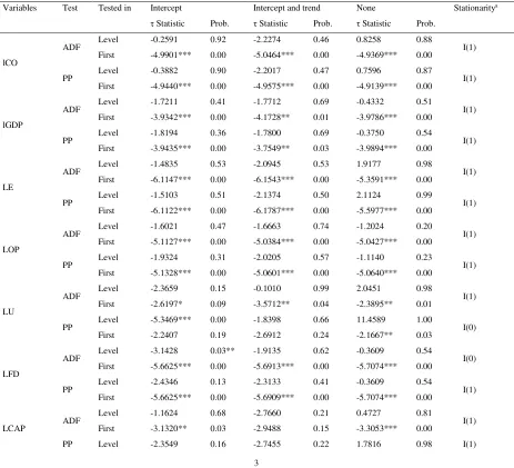
This study includes stationary tests (Dickey-Fuller and Pillips-Perron), cointegration test (Engle-Granger and Augmented Engle-Granger), rank and order condition tests, exogeneity tests, and three-stage least square estimation method whose results are as follows in the next paragraphs

Table 1- Stationarity tests results

Variables Test Tested in Intercept Intercept and trend None Stationaritya

τ _{Statistic Prob.} τ _{Statistic Prob.} τ _{Statistic Prob.}

lCO

ADF Level -0.2591 0.92 -2.2274 0.46 0.8258 0.88 I(1) First -4.9901*** 0.00 -5.0464*** 0.00 -4.9369*** 0.00

PP Level -0.3882 0.90 -2.2017 0.47 0.7596 0.87 I(1) First -4.9440*** 0.00 -4.9575*** 0.00 -4.9139*** 0.00

lGDP

ADF Level -1.7211 0.41 -1.7712 0.69 -0.4332 0.51 I(1) First -3.9342*** 0.00 -4.1728** 0.01 -3.9786*** 0.00

PP Level -1.8194 0.36 -1.7800 0.69 -0.3750 0.54 I(1) First -3.9435*** 0.00 -3.7549** 0.03 -3.9894*** 0.00

LE

ADF Level -1.4835 0.53 -2.0945 0.53 1.9177 0.98 I(1) First -6.1147*** 0.00 -6.1543*** 0.00 -5.3591*** 0.00

PP Level -1.5103 0.51 -2.1374 0.50 2.1124 0.99 I(1) First -6.1122*** 0.00 -6.1787*** 0.00 -5.5977*** 0.00

LOP

ADF Level -1.6021 0.47 -1.6663 0.74 -1.2024 0.20 I(1) First -5.1127*** 0.00 -5.0384*** 0.00 -5.0427*** 0.00

PP Level -1.9324 0.31 -2.0205 0.57 -1.1140 0.23 I(1) First -5.1328*** 0.00 -5.0601*** 0.00 -5.0640*** 0.00

LU

ADF Level -2.3659 0.15 -0.1010 0.99 2.0451 0.98 I(1) First -2.6197* 0.09 -3.5712** 0.04 -2.3895** 0.01

PP Level -5.3469*** 0.00 -1.8398 0.66 11.4589 1.00 I(0) First -2.2407 0.19 -2.6912 0.24 -2.1667** 0.03

LFD

ADF Level -3.1428 0.03** -1.9135 0.62 -0.3609 0.54 I(0) First -5.6625*** 0.00 -5.6913*** 0.00 -5.7074*** 0.00

PP Level -2.4346 0.13 -2.3133 0.41 -0.3609 0.54 I(1) First -5.6625*** 0.00 -5.6909*** 0.00 -5.7074*** 0.00

LCAP ADF

Level -1.1624 0.68 -2.7660 0.21 0.4727 0.81

I(1) First -3.1320** 0.03 -2.9488 0.15 -3.3053*** 0.00

4

First -3.1874** 0.02 -5.2973*** 0.00 -3.4144*** 0.00

LLAB

ADF Level -3.5767** 0.01 -3.4841** 0.05 -1.1093 0.23 I(0) First -3.0367** 0.04 -0.0858 0.99 -2.8290*** 0.00

PP Level -0.7881 0.81 -1.7261 0.71 0.4850 0.49 I(1) First -4.3566*** 0.00 -4.3848*** 0.00 -4.3895*** 0.00

*, **, and *** denote statistical significance at 10%, 5%, and 1% levels, respectively.

a _{I(x) shows the integration degree.}

Table 1 shows the results of the ADF and PP unit root tests with intercept, trend and intercept, and none of them in level and first difference. Based on the statistics, the integration degree of all the variables are identical, except for urban population, domestic credit to private sector, and labour force (which are stationary in level only by one of the two tests). The results, which show the identical integration degree, are statistically significant in one percent implying that all the variables can be cointegrated of degree one and have a long run relationship. So cointgration test is implemented

Tables 2- Engel and Granger (EG) and Augmented Engel and Granger (AEG) cointegration tests results Method Equation Test Intercept Intercept and

trend

None

τ Statistic Prob. τ Statistic Prob. τ Statistic Prob.

3SLS

(1) EG -3.6416 (0.00) -4.2177 (0.00) NA

AEG -4.3407 (0.00) -4.2356 (0.00) -4.4012 (0.00) (2) EG -3.7332 (0.00) -4.0829 (0.00) NA

AEG -4.1063 (0.00) -4.9984 (0.01) -4.1685 (0.00) (3) EG -4.0864 (0.00) -4.6305 (0.00) NA

AEG -4.8045 (0.00) -4.6633 (0.00) -4.8868 (0.00)

Table 2 indicates the results of the Engle-Granger and Augmented Engle-Granger cointegration tests. On the basis of table 2, the residuals of the three equations are stationary both in EG and AEG methods with statistically 1 percent significance. It implies that there is, at least, one linear combination among the variables which is stationary in level. Therefore, there is a long run relationship among the variables which confirms that the regression is not spurious. After performing the tests which are allocated to the variables, the system- or equation-related tests are implemented, the first of which is the order condition. The structural equations are as below:

(1)

= + + + + + +

(2)

= + + + + + + + +

(3)

= + + + + + + + +

Table 3- Order condition assessment No. of the variable

Order condition Identification Predetermined (K) Endogenous (M)

System 7 3

Equation (1) 3 3 − . > . −1 Over-identifiable

Equation (2) 5 3 − . = . −1 Just- identifiable

5

Table 3 represents the order condition of identification in simultaneous equations system. Based on the table, the number of exogenous variables included in the system but excluded from equation 1 is greater than the endogenous variables less than one. However, these two values are equal for the other two equations implying that, the first equation is over-identifiable while the other equations are just-identifiable. Consequently, the parameters of the system can be estimated.

Table 4- Variables’ coefficients arrangement Coefficients of the variables Equation

no. 1 (1) 1 0 0 0 0 (2) 1 0 0 (3) 1 0 0

Table 4 shows the coefficients of the three equations in a single matrix and table 5 presents whether the equations satisfies the rank conditions or not. There are six matrices, with none-zero determinants, ranked (2)×(2) and formed by the coefficients excluded from equation 1 but included in the system. Although the number of such matrix for the other equations is much less than six, there is one for each equation which implies that rank condition is satisfied for all the three equations. Therefore, both the order and rank conditions are satisfied for the system. The next step is to do the exogeneity test.

Table 5- Rank condition assessment.

Equation no. Matrices Rank condition

(1) 0

;

0

;

0

0 ;

;

0 ; and

0 Satisfied

(2) 0

Satisfied

(3) 0

Satisfied

Matrices of the coefficients of the variables excluded from the given equation but included in other equations which has non-zero determinants and ranked (M-1)×(M-1);M=3

Before estimating the system, exogeneity test is performed to assure that the endogenous variables are really endogenous, not seemingly. In order to perform the test, the reduced form of the simultaneous equations system should be established. Reduced forms of the equations whose dependant variables are suspect for endogeneity is as follows:

(4)

= + + + + + + + +

(5) = + + + + + + + +

6

(6) = + + + + + + + +

Table 6- Exogeneity test results

Equation Statistic Wald test = = 0 Null

hypothesis

Simultaneity hypothesis

Significance level Prob. Degree of freedom

(6) F-statistic 6.9461 0.00 2, 31 Rejected Accepted 1% Chi-square 13.8923 0.00 2 Rejected Accepted 1%

Table 6 shows the results of exogeneity test with both F-statistic and Chi-square. Both the statistics reject the null hypothesis of exogeneity of the variables. The statistics are much higher than the critical values and the null hypothesis is rejected in 1 percent level. It implies that both the suspected variables are really endogenous, not seemingly; and the system is specified correctly.

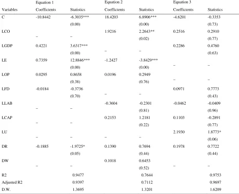
Table 7- Long run relationships and elasticities of the cointegrated simultaneous equations system

Equation 1 Equation 2 Equation 3

Variables Coefficients Statistics Coefficients Statistics Coefficients Statistics C -10.8442 -6.3035***

(0.00)

18.4203 6.8906*** (0.00)

-4.6201 -0.3353 (0.73) LCO

_ _ 1.9216 2.2643** (0.02)

0.2516 0.2910 (0.77) LGDP 0.4221 3.6317***

(0.00) _ _

0.2286 0.4760 (0.63) LE 0.7359 12.8846***

(0.00)

-1.2427 -3.8429***

(0.00) _ _ LOP 0.0295 0.8658

(0.38)

0.0196 0.2949

(0.76) _ _ LFD -0.0184 -0.3736

(0.70) _ _

0.0971 0.7773 (0.43) LLAB

_ _ -0.3604 -0.2301 (0.81)

-0.0462 -0.0409 (0.96) LCAP

_ _ 0.2153 1.2181 (0.22)

0.1103 -0.2891 (0.77) LU

_ _ _ _ 2.1930 1.8773* (0.06) DR -0.1885 -1.9725*

(0.05)

0.1390 0.7694 (0.44)

0.1978 0.7722 (0.44) DW

_ _ 0.1018 0.6453

(0.52) _ _ R2 0.9477 0.7644 0.9753 Adjusted R2 0.9397 0.7112 0.9697 D.W. 1.3695 1.3201 1.6209 *, **, and *** denote statistical significance at 10%, 5%, and 1% levels, respectively.

7

CO2 emissions, GDP, and energy consumption; in the third equation, the most effective one is urbanization. In the following paragraphs, it is explained how they affect the endogenous variables.

With regard to the column of the first equation, per capita GDP has a positive long run relationship with per capita CO2 emissions (0.4221) which is not only statistically significant in 1 percent level but also has the second greatest elasticity among the other elasticities. It implies that economic activities are the most extreme environmentally-pollutant factor after energy consumption which is consistent with Taghvaee and Parsa, 2014 and inconsistent with Taghvaee and Hajiani, 2015 and Baek, 2015. Likewise, per capita energy consumption has a positive long run relationship with per capita CO2 emissions (0.7359) which is not only statistically significant in 1 percent level but also has the greatest elasticity among the other coefficients, confirming that energy is the strongest environmentally-unfriendly factor which is consistent with Omri, 2013; Omri, 2014; Omri et al., 2015; Taghvaee and Hajiani, 2015; Al-mulali et al., 2015. Trade openness with 0.0259 has a positive long run relationship with CO2 emission, albeit statistically insignificant, indicating the positive effect of trade on environment pollution which is consistent with Omri, 2013; Omri, 2014; Omri et al., 2015. Financial development is related with CO2 emission negatively in long run (-0.0184), although statistically insignificant which is consistent with Jalil and Feridun, 2011; Shahbaz et al., 2013. Therefore, economic growth and energy consumption have the greatest impacts on the environmental pollution both in statistical significance and in value (positively) while the other variables have relatively lower elasticities which are statistically insignificant.

Based on the column of the second equation, per capita CO2 emission has a positive relation with per capita GDP with the greatest elasticity (1.9216) and statistically significance in long run, compared with the others. Trade openness (0.0196) and capital (0.2153) have the positive long run relationship with per capita GDP but not statistically significant. However, per capita energy consumption (-1.2427) and labour force (-0.3604) have negative long run relationships with per capita GDP with statistically significant and insignificant effects, respectively, coinciding with Omri 2013. Although energy and labour force are production factors, their coefficients are negative which can be due to decreasing or even reversing return to scale. Therefore, it is the capital that economy needs for growing in long run; not energy and labour.

With reference to the column of the third equation, all the variables show positive long run relationship but statistically insignificance, except labour force with negative coefficient and urban population with statistically significant effect in 10 percent level. Moreover, urban population has the greatest effect on energy consumption (2.1930) implying that, in long run, urbanization increases the level of per capita energy consumption which, in turn, is the most effective contributor to environmental pollution coinciding with Omri 2013. Therefore, urbanization is an environmentally-unfriendly element, acting through energy consumption increment.

All in all, per capita CO2 emissions, GDP, energy consumption show the strongest interactions (long run relationship and elasticities) in the equations system as a whole. So these three variables play the most important role in environmental, economic, and energetic decisions in long run. Besides, there is no doubt that urbanization indicates a noticeable effect on per capita energy consumption in the third equation.

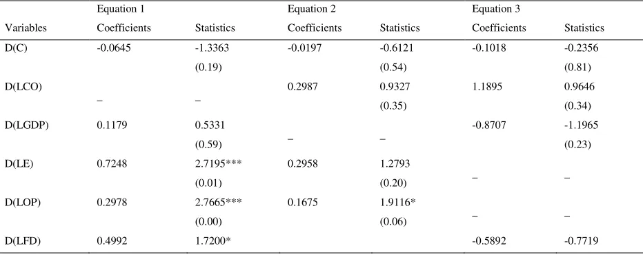
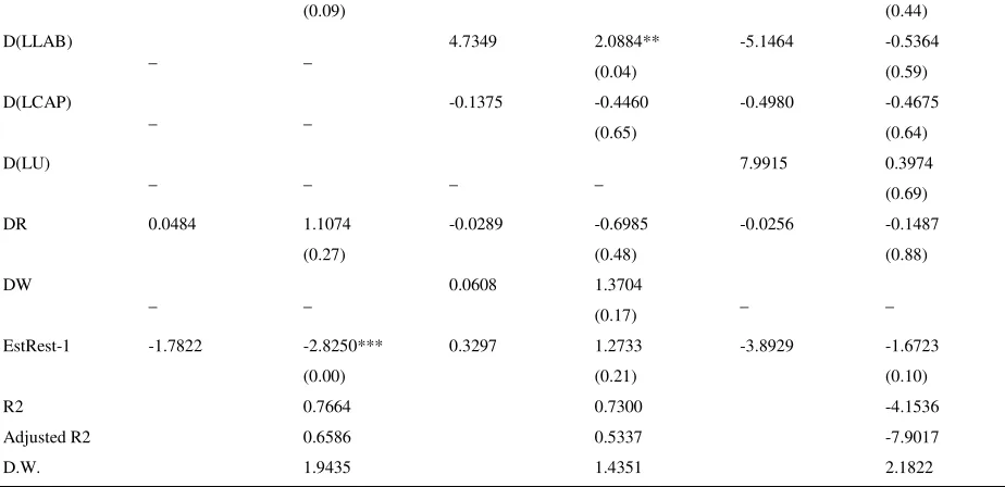
Table 8- Short run relationships and elasticities of the simultaneous equations system in error-correction model Equation 1 Equation 2 Equation 3

Variables Coefficients Statistics Coefficients Statistics Coefficients Statistics D(C) -0.0645 -1.3363

(0.19)

-0.0197 -0.6121 (0.54)

-0.1018 -0.2356 (0.81) D(LCO)

_ _ 0.2987 0.9327 (0.35)

1.1895 0.9646 (0.34) D(LGDP) 0.1179 0.5331

(0.59) _ _

-0.8707 -1.1965 (0.23) D(LE) 0.7248 2.7195***

(0.01)

0.2958 1.2793

(0.20) _ _ D(LOP) 0.2978 2.7665***

(0.00)

0.1675 1.9116*

8

(0.09) (0.44)

D(LLAB)

_ _ 4.7349 2.0884** (0.04)

-5.1464 -0.5364 (0.59) D(LCAP)

_ _ -0.1375 -0.4460 (0.65)

-0.4980 -0.4675 (0.64) D(LU)

_ _ _ _ 7.9915 0.3974 (0.69) DR 0.0484 1.1074

(0.27)

-0.0289 -0.6985 (0.48)

-0.0256 -0.1487 (0.88) DW

_ _ 0.0608 1.3704

(0.17) _ _ EstRest-1 -1.7822 -2.8250***

(0.00)

0.3297 1.2733 (0.21)

-3.8929 -1.6723 (0.10) R2 0.7664 0.7300 -4.1536 Adjusted R2 0.6586 0.5337 -7.9017 D.W. 1.9435 1.4351 2.1822 *, **, and *** denote statistical significance at 10%, 5%, and 1% levels, respectively.

Table 8 represents the three-stage least square estimation results of equations 4, 5, and 6 with coefficients, statistics, and probs. Since the variables are in natural logarithm, the coefficients can be construed as the elasticities: and due to the first differentiation of the variables, the coefficients can be interpreted as the short run relationships among the exogenous and endogenous variables. In contrast with the cointegrated equations, in the first two ECM equations, the most statistically-significant factors are trade openness, labour force, and financial development, rather than per capita CO2 emissions, GDP, and energy consumption (except per capita energy consumption in the first equation). The same as the third equation of the cointegrated equations, the most effective factor in the third ECM equation is urbanization, albeit statistically-insignificant. In the following paragraphs, the results of the three short run equations are explained one by one.

With regard to the first short run equation, all the variables have positive effects on the environmental pollution among which the most effective factors are per capita energy consumption, financial development, and trade openness. Per capita energy consumption shows the highest positive elasticity of CO2 emissions in short run (0.7248) which is statistically significant in one percent level. Financial development elasticity of environmental pollution (0.4992) takes the second greatest place in short run with statistical significance at ten percent, followed by trade openness elasticity (0.2978) with statistical significance at one percent. In sharp contrast to the cointegrated equation with the highest GDP elasticity of CO2 emissions, it is not only the least one in value (0.1179) but also the least one in statistical significance, although it is positive in both long run and short run. Notwithstanding the unexpected value of the lagged residuals coefficient (1.7822) which is greater than one, it is negative as expected. As a result, the highest short run elasticities of CO2 emissions are the lowest long run elasticities and vice versa.

Based on the column of the short run second equation, all the variables, except capital, have positive short run effects on economic growth among which the most effective factors are labour force and trade openness. In the short run, labour force elasticity of the economic growth is not only the largest one in value (4.7349) but also it is the most statistical significant (at five percent level). Despite the lower trade openness elasticity of economic growth in short run (0.1675), compared with those of CO2 emissions (0.2987) and energy consumption (0.2958), trade openness coefficient is statistically-significant (at 10 percent level) while those of CO2 emissions and energy consumption are not. Notwithstanding the expected value of the lagged residuals coefficient (0.3297) which is less than one, it is positive unexpectedly. Consequently, the driving forces of economic growth in the short run differ widely from those in the long run; as the labour force contributor is the biggest one in short run whilst the smallest one in the long run.

9

results of the third equation of the cointegrated model, the strongest negative elasticity is the labour force elasticity of energy consumption with -5.1464; and those of per capita GDP, financial development, and capital are the second, third, and forth strongest ones, respectively. Notwithstanding the unexpected value of the lagged residuals coefficient (-3.8929) which is greater than one, it is negative as expected. As a result, there are some similarities between the results of the third equations of the short run and long run models (such as the strongest effect of the urbanization in both models) and some differences (such as the effects of the labour force in the models which is the weakest and strongest one in the long run and short run models, respectively).

All in all, in the equations system as a whole, it is trade openness, labour force, financial development, and urbanization which show the most decisive effects in the short run, rather than per capita CO2 emissions, GDP, energy consumption (as in the long run). So the effectiveness of the system variables depends on the time period. Trade openness, labour force, and financial development play the most leading role in the short run, notwithstanding their limited role in the long run. However, energy consumption elasticity of CO2 emissions and urbanization elasticity of energy consumption are among the largest elasticities both in short run and long run.

4.Conclusion and Discussion

There are some implicit guidelines in the above results leading the policy makers to develop more sufficient and effective plans. Energy consumption, economic growth, urbanization, and trade openness are environmentally-unfriendly while financial development is environmentally-friendly factor.

Energy consumption is one of the most determining environmentally-unfriendly factors both in the short run and long run. Clearly, energy produces greenhouse and pollutant gases leading to increase the level of environmental pollution. So the governors should adopt some strategies to reduce the level of energy consumption, especially the fossil fuel ones such as oil, gasoline, diesel, and so forth, ignorant of whether they are deciding for the highest level of the management (long run) or the lowest (short run). Imposing or raising tax on energetic activities can be considered as a plan to reduce the level of energy consumption regardless of its negative effect on economic growth. Finally, energy consumption should be decreased by some policies both in short run and long run in order to decrease the environmental pollution.

Economic growth is another environmentally-unfriendly factor with a significant effect in the long run. Since Iran has a pollutant economy which is based on the fossil fuels, its economic growth leads to the environmental pollution. If the other economic sectors grow which are less pollutant, the economic growth may not increase the level of environmental pollution. As a result, the policy makers are advised to evolve the single-product economy into a multi-product one.

Urbanization is environmentally-unfriendly factor both in the long run and short run due to the energy-consuming mechanisms such as public transportation systems. The bigger the cities become, the more the energy is consumed which, in turn, leads to the more environmental pollution. The governors should increase the facilities needing for living in villages not only to stimulate the villagers to stay in their rural areas but also to tempt the citizens for moving and living in the countryside.

Trade openness has a positive effect on the environmental pollution. Although this effect is statistically-significant in the short run, it is insignificant in the long run. It implies that the changes in the trade policies quickly resulted in the environmental quality but the policy influence is faded out with the elapse of time in the long period of time. The decision makers should employ trade policies (such as customs tariffs and trade barriers) only for the emergency and critical situations to receive an immediate response.

Financial development has a negative effect on environmental pollution in the long run, albeit insignificant, owing to the fact that not only is it a green sector but also it can grow the sectors that improve the environmental quality in the longer periods of time. The policy makers in the higher management level (deciding on the policies with the long run effects) are advised to set a bigger budget to grow financial sector such as increasing the level of loans, credits, and investments, especially in the plans which are independent of energy like tourism plans. However, this effect is positive and significant in the short run which it suggests the deflation of financial development as an urgent treatment for the environmental pollution in the emergency and critical situations (just like the trade openness).

10

are influential for both the long run and short run policies. Examination of the relationship between the subsectors of financial and economic sectors and environmental pollution can be considered as a future study.

References

Al-Mulali, U., Saboori, B., Ozturk, I., 2015, Investigating the environmental Kuznets curve hypothesis in Vietnam, Energy Policy, 76, 123-131. Baek, J., 2015, Environmental Kuznets curve for CO2 emissions: The case of Arctic countries, Energy Economics, 50, 13-17.

Central Bank of the Islamic Republic of Iran, 2014. Economic time series database, Economic Research and Policy Department. Available from: < http://tsd.cbi.ir/>

Dickey, D. A., Fuller, W. A., 1979, distribution of the estimators for autoregressive time series with a unit root, Journal of the American Statistical Association, 74(366), 427-431

Engel, R.F., Granger, C.W.J., 1987.Co-intergration and error correction: representation, estimation and testing. Econometrica 55, 251-276.

http://dx.doi.org/10.2307/1913236

Ge, X., Li, Y., Luloff, A. E., Dong, K., Xiao, J., 2015, Effect of agricultureal economic growth on sandy desertification in Horqin Sandy Land, Ecological Economics, 119, 53-63

Grossman, G.M., Krueger A.B., 1991, Environmental Impact of a North American Free Trade Agreement, Working Paper 3914, National Bureau of Economic Research, Cambridge, MA.

Gujarati, D., (2004), “Basic Econometrics”, McGraw-Hill, 4th edition

Hao, Y., Zhang, Z., Liao, H., Wei, Y., 2015, China’s farewell to coal: a forecast of coal consumption through 2020, Energy Policy, 86, 444-455 Jalil, A., Feridun, M., 2011, The impact of growth, energy and financial development on the environment in China: a cointegration analysis, Energy

Economics, 33, 284-291.

Lee, S. and Oh D., 2015, Economic growth and the environment in China: empirical evidence using prefecture level data, China Economic Review, accepted manuscript

Lotfalipour, M. R., Falahi M. A., Ashena M., 2010, Economic growth, CO2 emissions, and fossil fuels consumption in Iran, Energy, 35, 5115-5120.

Omri, A., 2013, CO2 emissions, energy consumption and economic growth nexus in MENA countries: evidence from simultaneous equations model, Energy Economics, 40, 657-664.

Omri, A., 2014, Causal interactions between CO2 emissions, FDI, and economic growth: evidence from dynamic simultaneous-equation model, 42, 382-389.

Omri, A., Daly, S., Rault, C., Chaibi, A., 2015 Financial development, environmental quality, trade and economic growth: What causes what in MENA countries, Energy Economics, 48, 242-252.

Phillips, P. C. B., Perron, P., 1988, Testing for a unit root in time series regression, Biometrika, 75(2), 335-346.

Ren, S., Yuan, B., Ma, X., Chen, X., 2014, International trade, FDI (foreign direct investment) and embodied CO2 emissions: A case study of Chinas industrial sectors,

Report of the Intergovernmental Panel on Climate Change (IPCC), Yokohama, Japan, 2014

Shahbaz, M., Solarin, S., Mahmood, H., Arouri, M., 2013, Does financial development reduce CO2 emissions in Malaysian economy? A time series analysis, Economic Modelling, 35, 145-152.

Taghvaee, V. and Hajiani, P., 2014, Price and income elasticities of gasoline demand in Iran: using static, ECM, and dynamic models in short, intermediate, and long run. Modern Economy, 5, 939-950. doi:10.4236/me.2014.59087.

Taghvaee, V. M., Hajiani, P., 2015, Environment, Energy, and Environmental Productivity of Energy: A Decomposition Analysis in China and the US, Second European Academic Research Conference on Global Business, Economics, Finance and Banking, Zurich, Switzerland.

Taghvaee, V. M., Parsa, H., 2015, Economic growth and environmental pollution in Iran: Evidence from manufacturing and services sectors, Custos e Agronegocio Online, 11(1), 115-127.

Taghvaee, V.M., Shirazi, J.K., 2014, “Analysis of the relationship between economic growth and environmental pollution in Iran (Evidence from three sections of land, water and atmosphere)”. Indian Journal of Scientific Research, 7(1), 31-42.

World Bank, 2014, World Development Indicators.