Water Quality Sensor Model Based on an Optimization Method of RBF Neural Network

(1)

https://www.scirp.org/journal/cweee ISSN Online: 2168-1570

ISSN Print: 2168-1562

DOI: 10.4236/cweee.2020.91001 Nov, 19, 2019 1 Computational Water, Energy, and Environmental Engineering

Water Quality Sensor Model Based on an

Optimization Method of RBF Neural Network

Wei Huang

1

, Yiwei Yang

2

1_{Jiangsu Province Hydrology and Water Resources lnvestigation Bureau, Nanjing, China} 2_{China Union Pay Data Services Co. LTD, Shanghai, China}

Abstract

In order to solve the problem that the traditional radial basis function (RBF) neural network is easy to fall into local optimal and slow training speed in the data fusion of multi water quality sensors, an optimization method of RBF neural network based on improved cuckoo search (ICS) was proposed. The method uses RBF neural network to construct a fusion model for multiple water quality sensor data. RBF network can seek the best compromise be-tween complexity and learning ability, and relatively few parameters need to be set. By using ICS algorithm to find the best network parameters of RBF network, the obtained network model can realize the non-linear mapping be-tween input and output of data sample. The data fusion processing experiment was carried out based on the data released by Zhejiang province surface water quality automatic monitoring data system from March to April 2018. Com-pared with the traditional BP neural network, the experimental results show that the RBF neural network based on gradient descent (GD) and genetic al-gorithm (GA), the new method proposed in this paper can effectively fuse the water quality data and obtain higher classification accuracy of water quality.

Keywords

Water Quality Sensor, ICS Algorithm, RBF, Data Fusion, Nonlinear Mapping

1. Introduction

The problem of water resources pollution and shortage has become a major prob-lem in the development of social and economic development, so it is necessary to monitor the quality of water resources, measure the types of pollutants in wa-ter bodies, and concentrate of various pollutants and their changing trends, which provides reference data and basic means for water quality evaluation and predic-How to cite this paper: Huang, W. and

Yang, Y.W. (2020) Water Quality Sensor Model Based on an Optimization Method of RBF Neural Network. Computational Wa-ter, Energy, and Environmental Engineer-ing, 9, 1-11.

https://doi.org/10.4236/cweee.2020.91001

Received: September 24, 2019 Accepted: November 16, 2019 Published: November 19, 2019

(2)

DOI: 10.4236/cweee.2020.91001 2 Computational Water, Energy, and Environmental Engineering tion. However, the water quality data monitored by water quality sensors in the current automatic monitoring system is all single indicators, and there is no comprehensive evaluation of the monitored section water quality. According to the characteristics of the water quality data detected by the water quality moni-toring system, data fusion technology was introduced [1]. Since the data ob-tained by various water quality sensors is multi-source data, multi-source data fusion processing is required [2]. The neural network can provide an effective network model for data fusion because of its nonlinear mapping ability and strong self-learning ability. It has also achieved remarkable results in some prac-tical applications. Mahmood et al. proposed data fusion for different sensor mon-itoring data to improve the prediction ability of soil properties [3]. Qiu et al. proposed a multi-layer perceptron (MLP) data fusion algorithm based on ZigBee protocol architecture. The algorithm uses three layer perceptron models and im-proves the efficiency and total efficiency of the fusion of layers through the idea of cross layer fusion model [4]. Luciano et al. combines RBF neural network with genetic algorithm (GA) as cross-correlation method, and adopts multi-objective differential evolution and adaptive mode to optimize the network, which is used to predict swimmer’s velocity distribution [5].

In this paper, based on the structural features and nonlinear capability of RBF neural network, the data fusion algorithm of water quality sensor based on ICS optimization RBF is proposed. Cuckoo Search (CS) [6] is used to find the op-timal parameters of radial basis center, width and network weight, which solves the problem that the traditional training methods, such as gradient descent me-thod and PSO that are easy to fall into local optimal and slow training speed. The cuckoo algorithm is improved by using adaptive discovery probability and update step length, so that the optimal optimization of RBF network parameters can be achieved more accurately.

2. Water Quality Convergence Factors and

Classification Standards

2.1. Water Quality Convergence Factor

The classification of water quality parameters can be divided into biological, chem-ical and physchem-ical parameters based on biologchem-ical, chemchem-ical and physchem-ical cha-racteristics of water quality. Even if different water quality parameters are se-lected for fusion in the same water area, the final classification results may be different.

(3)

DOI: 10.4236/cweee.2020.91001 3 Computational Water, Energy, and Environmental Engineering

2.2. Classification Standard for Water Quality

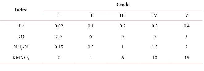
The classification criteria adopted in this paper are based on the Surface Water Environmental Quality Standard (GB3838-2002). According to the ground water uses purpose and protection target, surface water can be divided into five cate-gories, which have corresponding functions and purposes. The standard value of each basic item of surface water is divided into five categories, and the different functional categories implement the standard values of the corresponding cate-gories. The standard limits for the fusion factors total phosphorus, dissolved oxygen, ammonia nitrogen, and potassium permanganate used in this paper are shown in Table 1.

This standard is used as the basic standard for data fusion of multiple water quality sensors, and each category corresponds to one output unit of the RBF neural network.

3. Water Quality Sensor Data Fusion Algorithm

3.1. RBF Neural Network

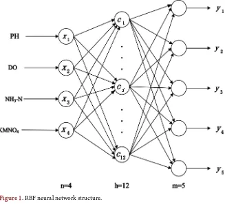
RBF neural network (RBF) is a three-layer feedforward neural network com-posed of single hidden layer, which has a strong ability to classify and approx-imate any nonlinear continuous function [7]. The number of hidden layer nodes, that is, the network structure, needs to be determined according to the specific problems of the study, so that the applicability of the network is better.

1) Determination of network structure

Since the number of input fusion factors is 4, the number of input layer nodes in the RBF neural network is 4. The output layer can be divided into five catego-ries according to the water quality category, so the number of output layer nodes is 5. There is no unified method for determining the number of nodes in the hidden layer. If the number of nodes is too large, the training time will be longer, the learning phenomenon will occur, and the network generalization ability and the prediction ability will decrease. Too few nodes result in less nonlinear ap-proximation ability and less fault tolerance. The commonly used empirical for-mula to determine the number of hidden layer nodes is:

h= n+ +m b (1)

[image:3.595.209.540.617.732.2]

where h is the number of hidden layer nodes, n is the number of input layer nodes,

Table 1. Surface water environmental quality standard.

Index Grade

I II III IV V

TP 0.02 0.1 0.2 0.3 0.4

DO 7.5 6 5 3 2

NH3-N 0.15 0.5 1 1.5 2

(4)

DOI: 10.4236/cweee.2020.91001 4 Computational Water, Energy, and Environmental Engineering and m is the number of output layer nodes, which is generally a constant of 1 to 10. We train the networks with 4 to 13 nodes respectively. The experimental re-sults show that the training error is the minimum when the number of hidden layer nodes is 12; therefore the number of hidden nodes is 12, which is the best number of nodes and has faster training speed and better generalization ability. The structure of the RBF neural network is shown in Figure 1.

The center of the hidden layer of the RBF neural network selects the Gaussian kernel function, then the output of the ith_{node of the output layer is:}

( )

2

1

1 exp

2 h

i ij j

j _j

y X ω X c

σ =

 

= _− − _

 

∑

(2)

where

{

}

T

1, 2, 3, 4

X = x x x x represents input from the input layer, ωij represents

the weight relationship between the ith_{node of the hidden layer and the}_jth_{node of}

the output layer. cj represents the node center of the hidden layer,

σ

j represents

the width of the hidden layer node. 2) Network training methods

RBF neural network parameters including the hidden layer nodes center cj,

the width of the hidden layer nodes σj and the weights between hidden layer

and output layer ωij, network parameters training method can have an

[image:4.595.213.540.430.727.2]

impor-tant impact on the performance of the network. Currently, the commonly used training methods are: clustering method [8], gradient descent method [9], ortho-gonal least squares algorithm (OLS) [10] [11], pseudo-inverse method and intel-ligent search algorithm. In order to solve the problem that the gradient descent

(5)

DOI: 10.4236/cweee.2020.91001 5 Computational Water, Energy, and Environmental Engineering method is easy to fall into local optimum and slow convergence, the ICS algo-rithm is used to optimize the network parameters.

3.2. Improved Cuckoo Search Algorithm

The CS algorithm is based on the behavior of cuckoo nest spawning and the characteristics of Levi’s flight. Three idealization criteria need to be assumed:

a) Each cuckoo produces only one egg at a time (that is, has an optimal solu-tion), and randomly selects a host bird’s nest;

b) In a randomly selected nest, only high-quality eggs will be hatched, and the corresponding optimal nest will remain in the next generation;

c) The number of host nests available in each iteration is fixed, and the proba-bility that the host bird nest finds alien cuckoo eggs is found. In this case, the host nest can destroy the egg or abandon the old nest and build a new one.

According to the above three criteria, there are two ways to update the nest position in cuckoo algorithm.

1) Update the position of the nest by Levy flight: Then, the updated formula of nest position is:

( ) (

)

1

, 1, 2, ,

t t

i i

x+ =x + ⊕α L λ i=  n

(3)

t i

x is the position of nest i in iteration t; n represents the number of nests; ⊕

represents the product of elements; α is the step size control factor, which con-trols the step size of random search, and the expression is:

(

)

0

t t

i best

x x

α α= −

₍₄₎

t best

x represents the best bird nest position in the tth iteration, and α0 is a

constant of 0.01 by default;

( )

L

λ

represents Levy’s random search step size, which is subject to Levy

distribution. When executing Levy flight according to Mantegna algorithm, the expression is [12]:

( )

1

u

L

v

β

λ

=

₍₅₎

1, 0 2

λ β= + < <β _, β_{affects the random search step size} L

( )

λ

, the default

value is 1.5; u and v are normally distributed.

2) Update the nest position by finding the probability pa:

The nest position updating formula is as follows:

(

)

(

)

1

t t t t

i i a j k

x

+

=

x

+

γ

H p

− ⊕

ε

x

−

x

(6)

γ_and ε_{obey the random number uniformly distributed between [0, 1],}

(

a

)

H p −

ε

is the Heviside function, which compares pa with the random

num-ber ε to control whether the nest position is updated. The function value is 0 when pa >ε, 0.5 when pa =ε, and 1 when pa<ε;

t j

x and xkt are

differ-ent random vectors in the tth_iteration.

(6)

DOI: 10.4236/cweee.2020.91001 6 Computational Water, Energy, and Environmental Engineering selected according to Levi’s flight and can easily jump from one area to another. It has a strong global search capability, but lacks local search capabilities. The fast convergence and precision of the standard CS algorithm cannot be guaran-teed. When pa is small and α is large, the number of iterations of the

algo-rithm searching for optimal parameters will increase significantly. When pa is

large and α is small, the algorithm converges rapidly, but the global optimal solution cannot be obtained [13]. To solve the problem of the standard CS algo-rithm, the parameter pa and step length parameter α were improved.

i) Adaptive discovery probability pa

Discovery probability pa is associated with the number of iterative steps. It

should gradually decrease as the number of iterations increases. At the initial stage, x should be a large value, and global optimization is carried out to increase the evolutionary strength and diversity of the population. At the end of the itera-tion, each nest is near the optimal soluitera-tion, and pa should be set to a smaller

value, which is conducive to convergence to the optimal solution, increase the probability of generating a new nest, and avoid falling into a local optimal solu-tion. The cosine function is introduced into the discovery probability, so that

a

p adaptively changes with the iteration:

(

)

min max min

1 cos 2 1 t a t

p p p p

T

π −

 

= + − × _ × _

−

  (7)

min

p _and pmax are respectively the minimum and maximum discovery

prob-ability, t is the number of current iterations, and T is the maximum number of iterations.

ii) Step parameter α adaptive update

The step size parameter α_{is related to the search precision of the algorithm,} and the step size should gradually decrease with the increase of the number of iterations. On this basis, for each nest in different iterations, different steps should be used to find new nests, and the fitness value of the nest is introduced into the step length update. The nest with poor fitness value can increase the step length to expand the search area and maintain the diversity of the nest. The nest with good fitness can be reduced so that it can search around the optimal value, which can accelerate the convergence speed. Therefore, the formula of step length up-date is:

(

)

max max min

t t i i t aver f t T f

α =_α − α −α × _×

 

(8)

min

α and αmax are respectively the minimum and maximum iteration step

sizes; t i

f is the fitness value of the ith nest at the tth iteration; favert is the

aver-age value of all nest fitness values in the tth_iteration.

( )

(

)

2

1

a

t t

i j j

j

f y x i

=

∑

− ₍₉₎

j

y represents the target value, and y represents the actual value obtained by

(7)

4. Algorithm Implementation Steps

The RBF neural network optimization method based on ICS can be divided into ICS algorithm part and RBF algorithm part. The part of the ICS algorithm mainly realizes the training and optimization of RBF network parameters, while the part of the RBF algorithm mainly obtains the parameters after the training of the ICS algorithm, and integrates and classifies the test sample data.

The algorithm implementation steps are as follows:

1) The structure of RBF neural network is first determined. The water quality data collected by the water quality sensor are preprocessed to determine the in-put sample data.

2) Randomly generate n nests. Each nest is composed of the hidden layer cen-ter of the RBF network. The width and the network weight of the hidden layer to the output layer, and is coded in the order of

[

c, ,

σ ω

]

, and each parameter of the ICS algorithm is set. Each nest is decoded, and the fitness value of each nest is calculated according to Formula (9) to obtain the minimum fitness value and the current optimal bird nest position.

3) Levy flight was used to update the position of the bird’s nest, that is, calcu-late the new bird’s nest position according to Equation (3) and calcucalcu-late the fit-ness value of the new bird’s nest.

4) Comparing the fitness value of the new bird nest with that of the old bird nest. If the fitness value of the new bird nest is smaller than that of the old bird nest, replace the old bird nest with a new one, and a group of better bird nests will be obtained.

5) A set of random Numbers is generated and compared with the discovery probability pa, and the solution larger than pa is eliminated, and the

corres-ponding quantity of new solutions is replaced according to Formula (6).

6) The fitness values of all updated nests were calculated, and the minimum fitness values and corresponding nest positions were found.

7) Determine the iterative termination condition. If the fitness value reaches the target accuracy or the iteration reaches the maximum number, stop the ite-ration and save the bird nest position corresponding to the current minimum fitness value. If the iteration condition is not satisfied, skip to step 3) to continue the iteration.

8) The final optimal bird nest is decoded as the radial basis, width and net-work weights of the hidden layer to the output layer of the RBF neural netnet-work.

9) Simulation experiments were conducted on the test samples.

5. Experimental Analysis

(8)

5.1. Parameter Settings

The number of nests n=10 was set in the RBF neural network optimization method based on ICS. The parameter β =1.5 that affects Levy’s search step size. Since the fitness value changes gradually as the probability of discovery be-comes smaller, the minimum and maximum discovery probabilities are set to

min 0.01

p = , pmax =0.6. According to the experiment in literature [14], the

maximum and minimum step length parameters αmax =0.5 and αmin =0.01

were set.

5.2. Experiment Analysis

In order to verify the convergence speed and the classification accuracy of test samples of the RBF neural network optimization method based on Improved Cuckoo Search (ICS), this Algorithm was compared with the classification Algo-rithm based on BP neural network, the RBF AlgoAlgo-rithm based on Gradient Des-cent (GD) and the RBF Algorithm based on Genetic Algorithm (GA). Because the algorithm proposed in this paper is to optimize the RBF neural network by improving the CS (ICS) algorithm, the proposed algorithm is recorded as ICS-RBF, the classification algorithm using BP neural network is recorded as BP, the RBF algorithm based on GD is recorded as GD-RBF, and RBF algorithm based on GA is recorded as GA-RBF. The performance of these algorithms is compared with the two indicators of fitness value change trained by RBF neural network and test sample prediction accuracy rate.

1) Fitness value

First, the fitness values of the RBF neural network are compared when the samples are trained, and the fitness value is the mean square error of the training sample target output and the actual output. The curve of fitness value change is shown in Figure 2.

It shows that the ICS-RBF algorithm has stronger global search and local search capabilities. When the number of iterations reaches 2000, the fitness value of GA-RBF algorithm is 0.2780, the fitness value of ICS-RBF algorithm was 0.2223, the fitness value of the GD-RBF algorithm is 0.3072, and the fitness value of the BP algorithm is 0.3402. Since the fitness value represents the error be-tween the target output and the actual output of training samples, the fitness value is smaller, which indicates that the prediction performance of RBF net-work for training samples is better. Therefore, the ICS-RBF algorithm has a bet-ter effect on the training of data samples. The trained RBF network model can more accurately predict the training samples and achieve a better non-linear fit-ting of the data samples to the output.

2) Prediction accuracy of test samples

(9)

com-DOI: 10.4236/cweee.2020.91001 9 Computational Water, Energy, and Environmental Engineering pared. Five groups of test sample data and actual sample prediction classification results were selected to compare and analysis. The selected test sample data is shown in Table 2.

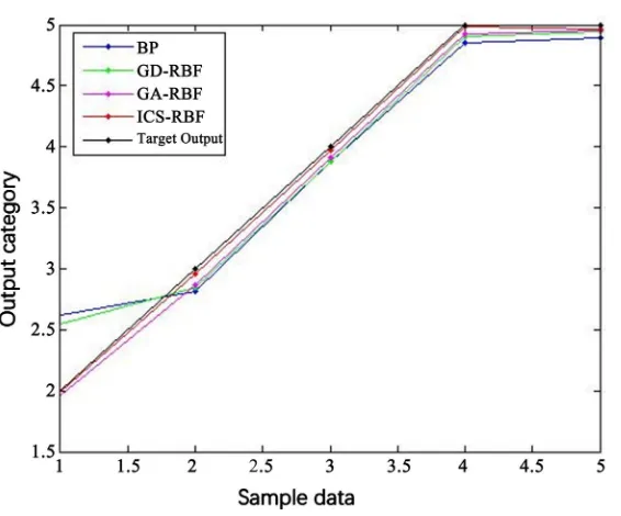
After the output results of the four RBF model prediction test samples are normalized, the maximum output probability obtained is added to the corres-ponding water quality category. The actual output results obtained are shown in Figure 3.

It shows that the predicted output result of RBF neural network based on the ICS algorithm is closer to the target output of the test sample, while the BP neural network model predicts the worst classification effect. When the BP and GD-RBF algorithms predict the data classification of the first group, the output prediction result is class II, which is inconsistent with the target result as class I. Therefore, compared with the other three models, the RBF network based on ICS algorithms has better effect on water quality data fusion processing, and the prediction results are closer to the actual results.

[image:9.595.228.518.341.572.2]

The prediction accuracy of the four network models for test samples is shown in Table 3.

[image:9.595.205.540.619.732.2]

Figure 2. Fitness curve.

Table 2. 5 groups of test sample data.

No. TP DO NH3-N KMNO4 Target output

1 0.016 9.97 0.07 0.71 [1, 0, 0, 0, 0]

2 0.099 8.00 0.10 4.50 [0, 1, 0, 0, 0]

3 0.036 3.25 0.61 3.5 [0, 0, 1, 0, 0]

4 0.234 4.67 1.30 7.79 [0, 0, 0, 1, 0]

(10)

[image:10.595.235.518.65.300.2]

DOI: 10.4236/cweee.2020.91001 10 Computational Water, Energy, and Environmental Engineering Figure 3. The actual output of the test sample.

Table 3. Predictive classification accuracy of test samples.

Method BP GD-RBF GA-RBF CS-RBF

Accuracy 72% 84% 86% 90%

It can be seen from the table that the accuracy of prediction and classification of water quality sensor data fusion based on ICS optimized RBF is 90%, which is 18% higher than that of BP neural network. The accuracy rate is 6% higher than that of RBF network based on GA, and the accuracy rate is 4% higher than that of the RBF network based on GA. Therefore, the optimization method achieved a better classification effect.

6. Conclusion

[image:10.595.206.537.346.380.2]

(11)

Conflicts of Interest

The authors declare no conflicts of interest regarding the publication of this pa-per.

References

[1] Yager, R.R. (2004) A Framework for Multi-Source Data Fusion. Elsevier Science Inc., Amsterdam.

[2] Wang, X., Xu, L.Z., Yu, H.Z., et al. (2017) Multi-Source Surveillance Information Fusion Technology and Application. Science.

[3] Mahmood, H.S., Hoogmoed, W.B. and Henten, E.J.V. (2012) Sensor Data Fusion t-o Predict Multiple Soil Properties. Precision Agriculture, 13, 628-645.

https://doi.org/10.1007/s11119-012-9280-7

[4] Qiu, J., Zhang, L., Fan, T., et al. (2016) Data Fusion Algorithm of Multilayer Neural Network by ZigBee Protocol Architecture. International Journal of Wireless & Mo-bile Computing, 10, 214-223.https://doi.org/10.1504/IJWMC.2016.077213

[5] Cruz, L.F.D., Freire, R.Z., Reynoso-Meza, G., et al. (2017) RBF Neural Network Combined with Self-Adaptive MODE and Genetic Algorithm to Identify Velocity Profile of Swimmers. Computational Intelligence, Athens, 6-9 December 2016, 1-7. [6] Yang, X.S. and Deb, S. (2010) Cuckoo Search via Levy Flights. World Congress on

Nature Biologically Inspired Computing, Coimbatore, 9-11 December 2009, 210-214. [7] Li, M.M. and Verma, B. (2016) Nonlinear Curve Fitting to Stopping Power Data

Using RBF Neural Networks. Expert Systems with Applications, 45, 161-171.

https://doi.org/10.1016/j.eswa.2015.09.033

[8] Karayiannis, N.B. and Mi, G.W. (1997) Growing Radial Basis Neural Networks: Merging Supervised and Unsupervised Learning with Network Growth Techniques.

IEEE Transactions on Neural Networks, 8, 1492.https://doi.org/10.1109/72.641471

[9] Naik, B., Nayak, J. and Behera, H.S. (2015) A Novel FLANN with a Hybrid PSO and GA Based Gradient Descent Learning for Classification. In: Proceedings of the 3rd International Conference on Frontiers of Intelligent Computing: Theory and Ap-plications, Springer, Cham, 745-754.https://doi.org/10.1007/978-3-319-11933-5_84

[10] Wang, N., Er, M.J. and Han, M. (2014) Parsimonious Extreme Learning Machine Using Recursive Orthogonal Least Squares. IEEE Transactions on Neural Networks and Learning Systems, 25, 1828-1841.https://doi.org/10.1109/TNNLS.2013.2296048

[11] Yang, Y.W. (2018) Research on Data fusion Algorithm of Water Quality Sensor. Ho-hai University, Nanjing.

[12] Mantegna, R.N. (1994) Fast, Accurate Algorithm for Numerical Simulation of Lévy Stable Stochastic Processes. Physical Review E: Statistical Physics Plasmas Fluids & Related Interdisciplinary Topics, 49, 4677.

https://doi.org/10.1103/PhysRevE.49.4677

[13] Valian, E., Tavakoli, S., Mohanna, S., et al. (2013) Improved Cuckoo Search for Re-liability Optimization Problems. Computers & Industrial Engineering, 64, 459-468.

https://doi.org/10.1016/j.cie.2012.07.011