Mode locking in a periodically forced "ghostbursting" neuron model

Mode locking in a periodically forced

“ghostbursting” neuron model

Carlo R. Laing

Institute of Information and Mathematical Sciences, Massey University, Private Bag 102-904, NSMC, Auckland, New Zealand

and

Stephen Coombes,

School of Mathematical Sciences, University of Nottingham, University Park, Nottingham, NG7 2RD, UK

April 7, 2004

Abstract: We study a minimal integrate-and-fire based model of a “ghostburst-ing” neuron under periodic stimulation. These neurons are involved in sensory processing in weakly electric fish. There exist regions in parameter space in which the model neuron is mode-locked to the stimulation. We analyse this locked be-havior and examine the bifurcations that define the boundaries of these regions. Due to the discontinuous nature of the flow, some of these bifurcations are non-smooth. This exact analysis is in excellent agreement with numerical simulations, and can be used to understand the response of such a model neuron to biologically realistic input.

1 Introduction

“Ghostbursting” is a novel type of neuronal bursting that has recently been charac-terised [Doiron et al., 2002]. It occurs in pyramidal cells in the electrosensory sys-tem of the weakly electric fishApteronotus leptorhynchus. These fish communicate, navigate and find prey using their electrosense. They generate a weak electric field with their electric organ (located in the tail) and sinusoidally modulate this in time at frequencies between approximately 800 and 1200 Hz. This electric field then permeates their local environment. Modulations in the amplitude and phase of the oscillation caused by nearby objects are detected by the fish’s electroreceptors, which cover the fish’s skin. These signals are then passed on to the electrosensory lateral line lobe (ELL) of the fish, and from there to higher brain centers.

In vitro studies of pyramidal cells from the ELL ofA. leptorhynchusshow that if a constant current (chosen from some appropriate interval) is injected into a cell, the cell’s action potentials are clustered together in bursts [Lemon & Turner, 2000]. These bursts are generated in an approximately periodic fashion, provided the injected current is kept fixed. Within a burst, the times between successive action potentials (spikes) monotonically decrease, i.e. the action potentials “speed up.” The end of a burst is marked by a very short interspike interval (ISI), which is followed by a long ISI, before the next burst commences. An example is shown in Fig. 1. This type of bursting (dubbed “ghostbursting”) was recently reproduced in a biophysically detailed model neuron [Doiron et al., 2001] and further analysed in a simpler yet still realistic model [Doiron et al., 2002].

One novel aspect of this type of bursting is that it seems necessary for the neu-ron undergoing bursting to be spatially extended, i.e. ghostbursting cannot be seen in a “point” neuron. This is apparent once the bursting mechanism is understood. In summary, both the pyramidal cell soma and dendrite are capable of producing spikes. Just after all but the last somatic spike in a burst, the dendrite fires a spike. During a burst there is a slow decrease in the dendritic potassium inactivation vari-able, causing the dendritic spikes to become wider in time, and causing the slow speed up of spikes — see Fig. 1. This speed up continues until the dendrite can no longer respond to a somatic spike (the dendritic refractory period is longer than that of the somatic). The lack of a dendritic spike then causes a long gap between two somatic spikes, during which the dendritic potassium inactivation variable increases, and another burst starts. See Doiron et al. [2002] for more details.

The model of Doiron et al. [2002] involves six nonlinear ODEs, which reproduce qualitatively, and to a large extent quantitatively, the experimentally observed bursting [Lemon & Turner, 2000]. Laing & Longtin [2002] introduced a minimal model of a ghostbursting neuron that had two variables, one “voltage” variable whose dynamics were governed by a modified integrate-and-fire mechanism, and a second variable that modulated the spike patterning so as to qualitatively repro-duce ghostbursting. It is that model that we study here, under periodic modulation of its input current.

than females, and when two fish are physically close the difference in EOD fre-quencies gives rise to a beat frequency, equal to that difference. Thus there are at least two types of periodic signals (the fish’s own EOD and the beat signal) that could be detected by electroreceptors on the fish’s skin and passed directly to the pyramidal cells that we are modelling. It is well known that weakly electric fish can detect beat frequencies, and change their own EOD frequency so as to increase the beat frequency [Zakon et al. 2002]. During such a jamming avoidance response the fish with the lower initial EOD frequency lowers its frequency while the other does the opposite, thereby increasing the beat rate to values that have little effect on electrolocation. This work can also be seen as a generalisation of work on peri-odically forced oscillators [Glass et al., 1984, Glass & Mackey, 1988].

Some work on the periodically forced ghostburster has been done previously [Laing & Longtin, 2002, Laing & Longtin, 2003]. Laing & Longtin [2002] studied the same model that we study here, but their analysis only allowed one to study mode-locked solutions in which the neuron fired once during a whole number of forcing periods, and they also ignored non-smooth bifurcations, whose study is es-sential for a complete understanding. Here we perform a full analysis of arbitrary mode-locked states for arbitrary periodic forcing, and investigate non-smooth bi-furcations of the system. Laing & Longtin [2003] studied the periodically forced neuron model consisting of six nonlinear ODEs presented by Doiron et al. [2002], but did not analyse mode-locked solutions in any detail.

The work presented here is similar to that in Coombes et al. [2001], where the authors analysed a periodically forced integrate-and-fire-or-burst neuron model. That model had a second variable to model a Ca2 _{ion current, and was capable of}

bursting under appropriate stimuli.

The structure of the rest of the paper is as follows. In Sec. 2 we present the discontinuous differential equations describing the minimal ghostbursting neu-ron and derive an implicit map for successive firing times. In Sec. 3 we describe mode-locked solutions and formulate a set of nonlinear simultaneous equations that any mode-locked solution must satisfy. Sec. 4 discusses the stability of these solutions and Sec. 5 shows some numerical results, comparing direct simulations with numerically determined resonance tongue boundaries. We summarize our main results in Sec. 6.

2 Model Equations

The differential equations describing our model neuron are

dV dt

A(t) V

c

∑

m n

H(tm tm 1

r) (t tm ) (1)

dc dt

c

(B

Cc2₎

∑

m n

(t tm) tn

t tn 1 (2)

with the rule V(t_n)

0 if V(t

n)

1, where H is the Heaviside step function and

This model was first introduced by Laing & Longtin [2002], although a redundant parameter in that formulation has been scaled out here.

Equations (1)-(2) define a modified integrate-and-fire (IF) neuron subject to periodic forcing. Periodically forced IF neuron models have been studied previ-ously [Keener et al., 1981, Coombes, 1999, Coombes & Bressloff, 1999], as have IF models with periodically varying [Glass, 1991] and dynamic [Chacron et al., 2003] thresholds.

The times tn are referred to as the firing times of the neuron. Between

fir-ing times, c decays exponentially to zero with time constant . At each firing

time, c is instantaneously updated c c

B

Cc2_{. Assuming that the last ISI}

(tn tn

1) was greater thanr, V is incremented by the value ofc at a time tn

.

If the last ISI was less than r, V is not incremented (this mimics the failure of the dendrite to respond to a somatic action potential). Typical “bursting” behavior of the system in shown in Fig. 2. The current is given by A(t)

I0

I1sin ( t).

Note that when I1

0, the system progressively moves from bursting to periodic firing and then quiescence as I0 is decreased, in agreement with experimental

ob-servations [Lemon & Turner, 2000] and the behavior of more sophisticated mod-els [Doiron et al., 2001, Doiron et al., 2002]. For more analysis of the model (1)-(2), see Laing & Longtin [2002].

Because (1)-(2) is piecewise linear, we can integrate overtn t tn 1to obtain

V(t;tn tn 1 cn)

G(t) e (t tn)

G(tn)

e (t tn)

H(t tn )H(tn tn 1

r)cne

ˆ

(3)

where 1 ˆ

1 1 , cn

c(t_n), and

G(t) 0

es_A(s

t)ds

The specific case we will study from now on is A(t)

I0

I1sin ( t), so

G(t)

I0

I1

1

2

[sin ( t) cos ( t)]

The next firing time,tn 1, is defined implicitly by

1

V(tn 1;tn tn 1 cn) (4)

wheretn 1is the smallest value greater thantnthat satisfies (4). We also have

cn 1 Ψ

(cn ∆n) (5)

where∆n

tn 1 tnand

Ψ(c t)

ce t

B

C ce t

2

(6)

previous ISI was shorter than the dendritic refractory period,r— and one resulting from the integration of the delta function in (1). The presence of these Heaviside functions can give rise to discontinuities in the solution, (3). We prefer to work with a smooth flow, so we can determine firing times by threshold crossings. We achieve this by replacing both Heaviside functions in (3) by

f (t) 1

1

e t

when necessary. Note that f (t) converges pointwise to H(t) as . For

nu-merical work, we set

100.

Together, (4) and (5) provide a means for calculating the sequence of firing times

tn , provided initial conditions are specified. We now discuss the existence of

mode-locked solutions.

3 Mode-locked Solutions

Mode-locked solutions are those for which the model neuron firesptimes for every

q periods of the forcing function, where p q . We refer to these solutions as

p:qmode-locked. For such solutions, the firing times are given by

tn n_p

n(p) q∆ n

0 1 2 (7)

where n(p)

n mod p, the

0

p 1

[0 1) are a collection of firing phases,

and [] denotes the integer part. Let us also define p

2 firing times

T 1

(

p 1

1)q∆ (8)

Tm

mq∆ 0 m p 1 (9)

Tp

(1

0)q∆ (10)

(These are just p

2 consecutive firing times, shifted so that all but the first and the last lie in the interval (0 q∆).) Substituting the firing times, (7), into (4) we see that the pfiring phases are determined by thepequations

1

Gn 1 e ∆n

Gn

e ∆n

H(∆n )H(∆n 1

r)cne

ˆ

n

0 p 1 (11)

whereGn

G(

nq∆) and∆n

Tn 1 Tn.

Thecnare given by (5)-(6), andc0satisfies

c0

Ψ( (Ψ(Ψ(c0 ∆0) ∆1) ) ∆p 1)

Ψ(cp 1 ∆p 1)

(12)

Thus we can find p: qmode-locked solutions by simultaneously solving the p

equations (11) and the single equation (12).

For periodically forced systems, there typically exist regions in parameter space in which mode-locked solutions exist, i.e. they are codimension-zero phenomena. These regions are called Arnol’d tongues and are often wedge-shaped, with one

point of the wedge touching a curve of zero forcing amplitude [Coombes & Bressloff, 1999, Glass, 1991]. The boundaries of these tongues are defined by instabilities of the

4 Stability

Here we examine the stability of mode-locked solutions. Introducing the notation

H(tn 1 tn tn 1)

H(tn 1 tn )H(tn tn 1

r), we can write each of the

equa-tions in (11) in the form

F(tn 1 tn tn 1 cn)

e∆n(G

n 1 1) Gn

H(tn 1 tn tn 1)cne ˆ 0 (13) where

cn 1

f(cn tn 1 tn)

Ψ(cn tn 1 tn) (14)

Considering perturbations of the formtn tn

nandcn cn

nabout a mode-locked solution gives a linearised system of equations:

0

F

tn 1

n 1 F tn n F

tn 1 n 1 F cn n (15) n 1 f

tn 1

n 1 f tn n f cn n (16)

where all partial derivatives are evaluated at the mode-locked solution. We can rewrite (15)-(16) as

n 1 n 1 n 1

Γn Φn Λn Φn Σn Φn

1 0 0

n n

n n n n n n n n (17)

where the coefficients are

Φn

F

tn 1

e∆n(A

n 1 1)

cne

ˆ

H

tn 1 (18)

Γn F tn An

cne

ˆ 1 tn H (19) Λn F

tn 1

cne

ˆ

H

tn 1

(20) Σn F cn e ˆ

H (21)

We have used the fact thatG(t)

A(t) G(t). The other coefficients are

n f tn Γn Φn f

tn 1 (22)

n Λn Φn f

tn 1 (23)

n f cn Σn Φn f

tn 1

Here An

A(Tn), and partial derivatives are given explicitly as

H

tn 1

H(∆n 1 r)H

(∆n

) (25) H tn

H(∆n )H (∆n

1

r) H(∆n 1

r)H (∆n

) (26)

H

tn 1

H(∆n )H (∆n

1

r) (27)

and f tn

cne ∆n

[1

2Ccne ∆n

] (28)

f

tn 1

f

tn (29)

f cn cn f tn (30)

Note that under the replacement of H(t) by f (t), we replace H(t) by f (t)[1

f (t)].

The stability of a p: q mode-locked state thus depends on the behavior of the map

un p

(p)un where un n n n and

(p)

p 1

p 2

0 (31)

If all of the eigenvalues of

(p) are less than one in magnitude, the corresponding mode-locked solution will be stable. Various bifurcations of the solution can occur when an eigenvalue of

(p) passes through the unit circle in the complex plane under variation of a parameter. Specifically, we expect a saddle-node bifurcation when

det(

(p) I)

0 (32)

where Iis the 3 3 identity matrix, a period-doubling bifurcation when

det(

(p)

I)

0 (33)

and a Neimark-Sacker bifurcation when

det(

(p))

1 (34)

provided the rank of

(p) is maximal [Wiggins, 1990]. As an example, it can be shown that det(

0 I)

0 when Φ0

Γ0

Λ0

0, and thus this equation can be used to find saddle-node bifurcations of 1 :q mode-locked solutions. It is interesting to note that the same equation would have been obtained if we had ignored perturbations in thecnwhen deriving

This linear stability analysis of the firing map will not detect bifurcations that occur when mode-locked solutions interact with discontinuities of the firing map. Indeed, we expect non-smooth bifurcations in such an integrate-and-fire system whenever a tangential crossing of the firing threshold occurs [Coombes et al., 2001]. We have observed a “grazing” bifurcation due to this phenomenon in the system under study, in which varying a parameter causes a subthreshold local maximum to increase through the firing theshold, leading to a new firing event that occurs at some time earlier than usual. For mode-locked solutions, these non-smooth bifur-cations are defined by

V(t ;tn tn 1 cn)

1 (35)

and

V(t ;tn tn 1 cn)

0 (36)

for sometn t tn 1, wheretn 1is the appropriate solution ofV(tn 1;tn tn 1 cn)

1. Note that from (3) we have

V(t;tn 1 tn cn)

V(t;tn 1 tn cn)

A(t)

e (t tn)

H(t

tn )H(tn tn 1

r)cne

ˆ

(37)

In principle there could also be a type of grazing bifurcation in which varying a parameter causes the voltage to reach the firing threshold but withdV dt

0 at that time, rather thandV dt

0 [Coombes et al., 2001]. This would also cause the solution to be lost in a non-smooth fashion and could be detected by appending the conditionV(tn)

0 to thep

1 equations defining the mode-locked orbit (11)-(12). However, we have not observed this type of bifurction in the system under study, so any subsequent discussion of grazing bifurcations will refer to the type described in the previous paragraph.

By considering both smooth bifurcations of the firing map and non-smooth bifurcations of the underlying discontinuous flow, we can construct the Arnol’d tongue structure of the periodically forced ghostbursting model neuron. For in-stabilities of the firing map (saddle-node, period-doubling and Neimark-Sacker bifurcations) we need to solve p

2 nonlinear algebraic equations (p

1 defining the molocked solution and one of (32)-(34)). For the grazing bifurcation de-scribed above we need to solve p

3 equations, the extra two being (35) and (36). For this type of bifurcation we need to take care with specifying between which two existing firing times the graze occurs.

In practice, numerical integration of (1)-(2) is used to determine approximate solutions of the simultaneous equations we wish to solve and these are used as initial guesses for Newton’s method. Once Newton’s method has converged we continue the solution in the appropriate system parameters using pseudoarclength continuation [Doedel et al., 1991].

5 Numerical Results

equations defining the edges of various Arnol’d tongues.

Figures 3, 6, 8 and 10 show the most positive Lyapunov exponent associated with the linearised map (17). This is one way of indicating the asymptotic behavior of the system at a particular point in parameter space. The maximal exponent is defined in the usual way:

lim n

1

nlog

(n)v (38)

where v is randomly chosen vector in

3 _and

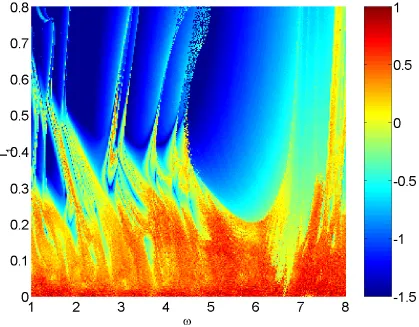
(n) is given in (31). At each point in these Figures, only one vector v was chosen to calculate , i.e. we did not av-erage several values of calculated using (38) with differentv’s. In some regions of these Figures there are “speckles” — this reflects multistability of the underly-ing dynamical system in these regions. At each point in the parameter plane the system (1)-(2) was integrated for 300 time units, and the first 10 firing times were ignored as transients.

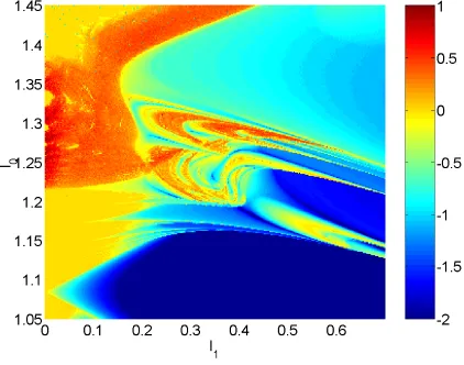
Figure 3 shows the maximal Lyapunov exponent as a function of both I0 and

I1 for

3. Other parameters are as in the caption of Fig. 2. We see that when

I1

0, i.e. there is no temporal modulation of the input current, the model moves from periodic (

0) to chaotic (

0) behavior as I0 increases through

approx-imately 122. In fact, the model moves from periodic firing to bursting, which

is known to be chaotic [Laing & Longtin, 2002]. It can also be seen from Fig. 3 that when I1

0 and I0 is greater than about 138, the system behaves

period-ically. In this parameter region the model neuron is firing “doublets” — alter-nating long and short ISIs — behavior seen in other models of this type of neu-ron [Doineu-ron et al., 2002, Laing & Longtin, 2002]. Also, when I1

0, the frequency of firing for I0 1

22 increases as I0 is increased. Thus we see Arnol’d tongues

emanating from the I0axis, the largest being the 1 : 1 tongue.

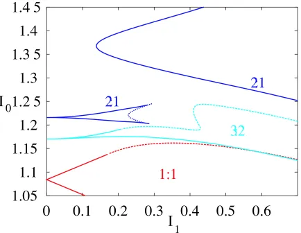
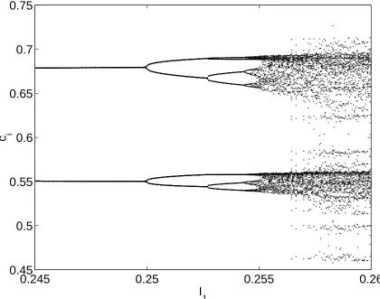
In Fig. 4 we see boundaries of several tongues, calculated using the ideas pre-sented in Sec. 4. Here, as in other Figures, the Arnol’d tongues are constructed from the union of smooth bifurcations of the firing map and non-smooth bifurcations of the underlying discontinuous flow. Neither Neimark-Sacker nor period-doubling bifurcations seem to play a large role in the determination of the tongue struc-ture, although both are present. For example, there is period-doubling within the 2 : 1 tongue shown in Fig. 4, and a horizontal slice through this Figure at I0

122

is shown in Fig. 5. The first few period-doublings can be seen, which strongly suggests that the system may pass through a period-doubling cascade to chaotic behavior as parameters are varied. Neimark-Sacker bifurcations have previously been found for this model and are discussed by Laing & Longtin [2002]. It is in-teresting to note that the 2 : 1 border of Fig. 4 has two distinct pieces. Moreover, within the upper 2 : 1 border we find 2(q

1) : (q

1) solutions that bifurcate in turn from 2q:qsolutions as one moves deeper into the interior of the 2 : 1 tongue. In this, and indeed all Arnol’d tongue diagrams, we find excellent agreement be-tween theory and direct numerical simulations.

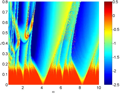
In Fig. 6 we show the maximal Lyapunov exponent as a function of and I1for

I0

125. From Fig. 3 we see that when I1

0 and I0

125, the system is

the forcing can move the system from chaotic behavior to periodic, by forcing it to become mode locked to the forcing. The minimum amplitude required for this de-pends on the frequency of forcing. In Fig. 7 we plot the corresponding boundaries of several tongues shown in Fig. 6.

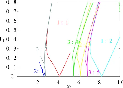
Figure 8 also shows the maximal Lyapunov exponent in the ( I1) plane, but for

I0

115. For this value of I0, the system fires periodically whenI1

0, in contrast to the case shown in Fig 6. Here we clearly see Arnol’d tongues emanating from the zero forcing amplitude line. The corresponding theoretical Arnol’d tongue structure is shown in Fig. 9, and nicely illustrates another organizing feature of the Arnol’d tongues; namely that those emanating from the zero forcing amplitude line are arranged such that between a p: q and a p : q tongue one can expect to

see a p

p :q

q tongue.

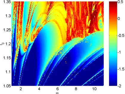
Figure 10 shows the maximal Lyapunov exponent as a function of both and

I0 for I1

04. Recalling that when I1

0, the system switches from periodic to chaotic firing at I0 122, we see that the nonzero forcing amplitude can either

delay the onset of chaotic behavior as I0 is increased (for example, when

5) or hasten it (for example, when 7). Finally in Fig. 11 we plot the

correspond-ing Arnol’d tongue structure for Fig. 10. For these parameter values we note the extensive overlap of tongue borders, highlighting the multi-stable nature of mode-locked solutions, thus accounting for the speckled nature of Fig. 10.

6 Discussion

We have exactly analysed the response of a model ghostbursting neuron to an ar-bitrary periodic modulation of its input current, and compared these results with those from numerical integration of the model undergoing sinusoidal forcing. The agreement is very good. Despite the fact that the unforced system undergoes a bifurcation from periodic firing to chaotic bursting as the injected current is in-creased, its behavior when periodically forced can be largely understood by trac-ing boundaries of Arnol’d tongues. The boundaries of these tongues correspond to either local bifurcations of the firing time map, or non-smooth bifurcations of the underlying flow, caused by its discontinuous nature.

List of Figures

1 An example of “ghostbursting” in the model of Doiron et al. [2002]. The somatic voltage is shown as a function of time. Note the pro-gressive shortening of successive ISIs during each burst, and the large ISIs that separate bursts. The injected current is I

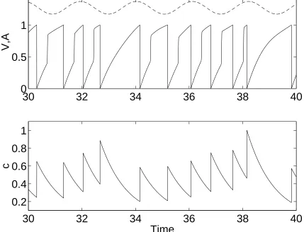
10; other parameters are as in Doiron et al. [2002]. . . 14 2 Typical behavior of the model (1)-(2). The top panel showsA(dashed)

and V(solid), while the lower showsc. The neuron “fires” whenV

reaches 1 from below. Compare with Fig. 1. Parameter values are

B

035 C

09

1

04 r

07 I0

127 I1

01

3. . . 15 3 Maximal Lyapunov exponent (color coded) as a function of I0 and

I1, on a mesh of size 300 300, for

3. Other parameters are as in the caption of Fig. 2. . . 16 4 Arnol’d tongue diagram corresponding to Fig. 3, for a 1 : 1

mode-locked solution (red), 2 : 1 solution (dark blue) and a 3 : 2 solution (light blue) Solid lines indicate a saddle-node bifurcation of the fir-ing map and dashed lines a non-smooth grazfir-ing bifurcation of the underlying flow. The dotted line indicates a period-doubling bifur-cation of the 2 : 1 orbit (see Fig. 5). Note that there are two distinct 2 : 1 tongues. . . 17 5 This shows 50 successive values ofciat each value ofI1, forI0

122

and

3. The first few period-doublings are clear. Compare with Fig. 4. . . 18 6 Maximal Lyapunov exponent (color coded) as a function of and I1

for I0

125. Other parameters are as in the caption of Fig. 2. . . 19

7 Arnol’d tongue diagram corresponding to Fig. 6, for a 1 : 1 mode-locked solution (red), 3 : 1 solution (dark blue) and a 3 : 2 solution (light blue). . . 20 8 Maximal Lyapunov exponent (color coded) as a function of and

I1 for I0

115. Other parameters are as in the caption of Fig. 2.

Compare with Fig. 6. . . 21 9 Corresponding Arnol’d tongue structure for Fig. 8. Note that

be-tween a p:qand ap :q tongue one can expect to see a p

p :q

q

tongue, for low amplitude forcing. . . 22 10 Maximal Lyapunov exponent (color coded) as a function of and I0

for I1

04. Other parameters are as in the caption of Fig. 2. . . 23

References

[Chacron et al., 2003] Chacron, M. J., Pakdaman, K. & Longtin, A. [2003] “Inter-spike interval correlations, memory, adaptation, and refractoriness in a leaky integrate-and-fire model with threshold fatigue”,Neural Comput.15, 253-278.

[Coombes, 1999] Coombes, S. [1999]. “ Liapunov exponents and mode-locked so-lutions for integrate-and-fire dynamical systems,”Phys. Lett. A255, 49-57.

[Coombes & Bressloff, 1999] Coombes, S. & Bressloff, P. C. [1999]. “Mode locking and Arnold tongues in integrate-and-fire neural oscillators,” Phys. Rev. E 60, 2086-2096.

[Coombes et al., 2001] Coombes, S., Owen, M. R. & Smith, G. D. [2001]. “Mode locking in a periodically forced integrate-and-fire-or-burst neuron model,”Phys. Rev. E64, 041914.

[Doedel et al., 1991] Doedel, E., Keller, H. B. & Kernevez, J. P. [1991] “Numerical analysis and control of bifurcation problems. I: Bifurcation in finite dimensions,”

Int. J. Bif. Chaos1, 493-520.

[Doiron et al., 2001] Doiron, B., Longtin, A., Turner, R. W. & Maler, L. [2001]. “Model of gamma frequency burst discharge generated by conditional back-propagation,”J. Neurophysiol.86, 1523-1545.

[Doiron et al., 2002] Doiron, B., Laing, C. R., Longtin, A. & Maler, L. [2002]. ““Ghostbursting”: a novel bursting mechanism in pyramidal cells,” J. Comput. Neurosci.12, 5-25.

[Glass et al., 1984] Glass, L., Guevara, M. R., Belair, J. & A. Shrier , [1984]. “Global bifurcations of a periodically forced biological oscillator,”Phys. Rev. A29, 1348-1357.

[Glass, 1991] Glass, L. [1991]. “Cardiac arrhythmias and circle maps – a classical problem,”Chaos1, 13-19.

[Glass & Mackey, 1988] Glass, L. & Mackey, M. C. [1988]. From Clocks to Chaos

(Princeton University Press).

[Izhikevich, 2000] Izhikevich, E. M. [2000]. “Neural excitability, spiking and burst-ing,”Int. J. Bifn. Chaos10, 1171-1266.

[Keener et al., 1981] Keener, J. P., Hoppensteadt, F.C., & Rinzel, J. [1981]. “Integrate-and-fire models of nerve membrane response to oscillatory input,”

SIAM J. Appl. Math.41, 816-823

[Laing & Longtin, 2003] Laing, C. R. & Longtin, A. [2003]. “Periodic forcing of a model sensory neuron,”Phys. Rev. E67, 051928.

[Lemon & Turner, 2000] Lemon, N. & Turner, R. W. [2000]. “Conditional spike backpropagation generates burst discharge in a sensory neuron,” J. Neurophys-iol.841519-1530.

[Wiggins, 1990] Wiggins, S. [1990].Introduction to Applied Nonlinear Dynamical Sys-tems and Chaos,(Springer-Verlag, New York).

[Zakon et al. 2002] Zakon, H., Oestreich J., Tallarovic S., & Triefenbach F. [2002]. “EOD modulations of brown ghost electric fish: JARs, chirps, rises, and dips,”

0

10

20

30

40

50

60

70

−80

−60

−40

−20

0

20

40

Time (ms)

V (mV)

Figure 1: An example of “ghostbursting” in the model of Doiron et al. [2002]. The somatic voltage is shown as a function of time. Note the progressive shortening of successive ISIs during each burst, and the large ISIs that separate bursts. The injected current is I

30

32

34

36

38

40

0

0.5

1

V,A

30

32

34

36

38

40

0.2

0.4

0.6

0.8

1

Time

c

Figure 2: Typical behavior of the model (1)-(2). The top panel shows A(dashed) andV(solid), while the lower showsc. The neuron “fires” whenVreaches 1 from below. Compare with Fig. 1. Parameter values are B

035 C

09

1

04 r

07 I0

127 I1

01

Figure 3: Maximal Lyapunov exponent (color coded) as a function of I0and I1, on

a mesh of size 300 300, for

1.05

1.1

1.15

1.2

1.25

1.3

1.35

1.4

1.45

0

0.1

0.2

0.3

0.4

0.5

0.6

Ι

0

Ι

1

1:1

3:2

2:1

2:1

0.245

0.25

0.255

0.26

0.45

0.5

0.55

0.6

0.65

0.7

0.75

I

c

Figure 5: This shows 50 successive values ofciat each value ofI1, for I0

122 and

Figure 6: Maximal Lyapunov exponent (color coded) as a function of and I1for

I0

0

0.1

0.2

0.3

0.4

0.5

0.6

0.7

0.8

1

2

3

4

5

6

7

8

1:1

ω

I

1

3:2

3:1

Figure 8: Maximal Lyapunov exponent (color coded) as a function of and I1for

I0

0

0.1

0.2

0.3

0.4

0.5

0.6

0.7

0.8

2

4

6

8

10

ω

I

₁

1:2

3:5

2:3

3:4

1:1

3:2

2:1

Figure 9: Corresponding Arnol’d tongue structure for Fig. 8. Note that between a p : q and a p : q tongue one can expect to see a p

p : q

q tongue, for low

Figure 10: Maximal Lyapunov exponent (color coded) as a function of and I0for

I1

1.05

1.1

1.15

1.2

1.25

1.3

1.35

2

4

6

8

10

ω

I

₀

3:1

2:1

1:1

2:3

1:2

1:3