Online Full Text

(1)

Abstract—A family of transformations is the one of several methods to analyze the data that do not correspond with the assumption. A well-known family of transformations often used in many studies was proposed by Box and Cox. However, Box-Cox transformation is not always applicable. It should be used with caution in some cases such as failure time and survival data. The simple case, some observations in the set of failure time data may be zero but the value of observation in the condition of Box-Cox transformation is greater than zero. In this case, Manly transformation may be appropriated than Box-Cox transformation because it was proposed as a family of exponential transformations that negative x values are also allowed. In this paper, a new family of transformation is proposed to manage with the problem as mentioned and Manly transformation were compared in the lifetime data those have exponential gamma and weibull distribution. They were investigated for some sets of the lifetime data. It is found that the proposed transformation and Manly transformation have not different efficiency in

sense of normality. The proposed transformation performs better than Manly transformation in

sense of homogeneity of variances for some data set of weibull distributions and exponential distributions when the sample sizes are large.

Index Terms— Manly transformation, proposed

transformation, homogeneity of variances, lifetime data,

normality

I. INTRODUCTION

N statistical data analysis, many statistical procedures require data to be approximately normal. If the data are not normally distributed, a transformation that transforms the data set to achieve normality is used. Tukey [1] suggested that when analyzing data that do not match the assumptions of a conventional method of analysis, there are two choices; transform the data to fit the assumptions or develop some new robust methods of analysis. Montgomery

Manuscript received February 24, 2014; revised March 17, 2014. This work was supported in part by the Faculty of Science, Maejo University, Chiang Mai, Thailand.

L. Watthanacheewakul is with the Faculty of Science, Maejo University, Chiang Mai, Thailand (phone: 66-53-873-551; fax: 66-53-875-205; e-mail: [email protected]; [email protected]).

[2] suggested that transformations are used for three purposes; stabilizing response variance, making the distribution of the response variable closer to a normal distribution and improving the fit of the model to the data. There are several alternatives for transforming such as transformations based on the relationship between the standard deviation and the mean. Furthermore, it is possible to transform the data using a family of transformations already extensively studied over a long period of time, e.g. Box and Cox [3], Manly [4], and John and Draper [5] . A well-known family of transformations often used in previous studies was proposed by Box and Cox. Doksum and Wong [6] indicated that the Box-Cox transformation should be used with caution in some cases such as failure time and survival data.John and Draper [5] showed that the Box-Cox transformation was not satisfactory even when the best value of transformation parameter had been chosen.

II. AFAMILY OF TRANSFORMATIONS

A family of transformations applied over a long period can be used for data from any population so that the transformed data are normally distributed.

Let X be a random variable distributed as non-normal,Y the transformed variable of X, x the value of X, c the range of data set and λ a transformation parameter.

Box and Cox [3] gave a simple modified form of the power transformation to avoid discontinuity at λ=0. They considered

1 , 0 ln , 0

⎧ − _≠

⎪ = ⎨

⎪ ₌

⎩ X Y

X λ

λ λ

λ

for . (1)

This has become well known as Box-Cox transformation. Manly [4] suggested a one parameter family of exponential transformations

exp( ) 1

, 0

, 0.

−

⎧ _≠

⎪ = ⎨

⎪ ₌

⎩ X Y

X

λ _λ

λ

(2)

This is a useful alternative to Box-Cox transformations because negative x values are also allowed. It has been

x 0

>

A New Family of Transformations for

Lifetime Data

Lakhana Watthanacheewakul

(2)

found in particular that this transformation is quite effective at turning skew unimodal distributions into nearly symmetric normal distributions.

Yeo and Johnson [8] proposed a family of modified Box and Cox transformation

[

]

[

]

[

]

[

]

1 1

, 0, 0

ln 1 , 0, 0

1 1

, 0, 0

ln 1 , 0, 0

⎧ ₊ ₋ ⎪ ≥ ≠ ⎪ ⎪ ₊ _≥ ₌ ⎪ = ⎨ + − ⎪ < ≠ ⎪ ⎪

⎪ + < =

⎩ X x X x Y X x X x λ λ λ λ λ λ λ λ (3)

In this paper, the alternative family of transformations for lifetime data is proposed in this form

1 1

, 0, 0

ln 1 , 0, 0.

⎧⎡_⎣ + ⎤_⎦ − ⎪ _≥ _≠ ⎪ = ⎨ ⎪ ⎡ + ⎤ ≥ = ⎪ ⎣ ⎦ ⎩ X x Y X x λ λ λ λ (4)

III. LIFETIME DATA

Lifetime data are important in reliability analysis and survival analysis. It is often of interest to estimate the reliability of the system/component from the observed lifetime data.

Weibull Exponential and Gamma distributions are involved lifetime data. The Weibull distribution is a natural starting point in the modeling of failure times in reliability, material strength data and many other applications. The probability density function of a two parameter Weibull random variable X is

1

, 0; , 0

( )

0 , <0

− ⎛ ⎞ −⎜ ⎟ ⎝ ⎠

⎧ ⎛ ⎞

⎪ _{⎜ ⎟} _≥ _>

= ⎨ ⎝ ⎠ ⎪ ⎩ x x e x f x x α α β

α _{α β}

β β ’ (5)

where α is the shape parameter and β is the scale parameter. It is related to the other probability distribution such as the Exponential distribution when α=1. The probability density function of one parameter Exponential random variable X is

1

, 0; 0

( )

0 , <0

⎛ ⎞ −⎜ ⎟ ⎝ ⎠

⎧

⎪ ≥ >

= ⎨ ⎪ ⎩ x e x f x x β _β

β ’ (6)

where β is the scale parameter.

Gamma distribution is the common choices of frailty distribution in lifetime data models.

1 1

, 0; 0

( ) _{( )}

0 , <0

⎛ ⎞ −⎜ ⎟ − ⎝ ⎠

⎧

⎪ ≥ >

= ⎨ Γ ⎪ ⎩

x

x e x

f x

x β α

α β

β α (7)

where α is the shape parameter and β is the scale parameter.

IV. ESTIMATION OF THE TRANSFORMATION PARAMETER For several groups of data, the value of λ in (2) and (3) need to be found so that the transformed variables will be independently normal distribution with homogeneity of variances. The probability density function of each Yij is in

the form

2 2

1 2

2 2

1 1

( , ) exp ( )

2 (2 )

⎧ ⎫

= _⎨− − _⎬

⎩ ⎭

ij i ij i

f y μ σ y μ

σ

πσ , (8)

where μi is the mean of the ith transformed population data,

2

σ the pooled variance of all transformed population data and yij the observed value of Yij. For (2), the likelihood

function in relation to the observations xij is given by

2

2 2 ₁ ₁

( , , )

exp( ) 1

1 1

exp . ( ; )

2

(2 ) = =

= ⎧ _⎡ ₋ _⎤ ⎫ ⎪₋ ₋ ⎪ ⎨ ⎢ ⎥ ⎬ ⎣ ⎦ ⎪ ⎪ ⎩

∑∑

⎭ i i ij n k ij i n i j L x x

J y x

μ σ λ

λ μ σ λ πσ (9) where 1 1 ( ; ) = = ∂ = ∂

∏∏

k ni

ij

i j ij

y J y x

x . For a fixed λ, the MLE’s forμi and

2

σ are

1

exp( ) 1

1 ˆ = − ⎡ ⎤ = _⎢ _⎥ ⎣ ⎦

∑

ni

ij i j i x n λ μ

λ and

2 2

1 1 1

exp( ) 1 exp( ) 1

1 1 ˆ = = = ⎧ − ⎛ − ⎫⎞ ⎪ ⎪ = ⎨ − ⎜ ⎟⎬ ⎪ ⎝ ⎠⎪ ⎩ ⎭

∑∑

k ni

∑

ni

ij ij

i j i j

x x

n n

λ λ

σ

λ λ

Substitute ˆμiand

2 ˆ

σ into the likelihood equation (9). Thus for fixed λ, the maximized log likelihood is

2

1 1 1

1 1 ln ( )

exp( ) 1 exp( ) 1

1 1

ln 2 ln

2 2 2 = = = = = = ⎧ − ⎛ − ⎞⎫ ⎪ ⎪ − − _⎨ − _⎜ _⎟_⎬ ⎪ ⎝ ⎠⎪ ⎩ ⎭ +

∑∑

∑

∑∑

i i i ij n n k ij ij

i j i j

n k ij i j L x x x n n n n n x λ λ λ π λ λ λ - , (10) except for a constant, the maximum likelihood estimate of

λ

is obtained by solving the likelihood equation

( )

2

1 1 1 1 1

2 2

1 1 1 1

1 1 ln 1 1 0. = = = = = = = = = = = = ⎡ ⎛ ⎞⎛ ⎞⎤ − ⎢ − ⎜ ⎟⎜ ⎟⎥ ⎢ ⎝ ⎠⎝ ⎠⎥ ⎣ ⎦ ⎛ ⎞ − _⎜ _⎟ ⎝ ⎠ + + =

∑∑

∑ ∑

∑

∑∑

∑ ∑

∑∑

i i i

ij ij ij

i i

ij ij

i

n n n

k k

x x x

ij ij

i j i i j j

n n

k k

x x

i j i i j

n k ij i j d L d

n e x e e x

n

e e

n

x

λ λ λ

λ λ λ λ λ (11) Similar procedures yield the same results for (4), the

(3)

co m th th fu nu va tra si = an an pa be W Fi Fig

(

1 1 1 1 1 ln 1 = = = = = ⎡ ⎢ ⎢ − ⎢ ⎢ ⎢⎣ + +

∑∑

∑

∑∑

i n k i j k i i k i j k i j d L d n n n λ λ λ

Since λappe onsidered to maximized log

he value of th he slope of th unction is ne umerical meth alue of λ.

In order to ansformations gnificant valu 3, ni= samp

nd 80, βi= sc

nd Gamma p arameter of t etween 2 and Weibull Expon

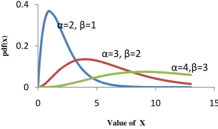
igure 1 – 7.

g. 1. Graph of W same and s

0 0.2 0.4 0.6 0.8 1 0 pdf(x)

)

(

)

(

)

(

)

(

2 1 2 1 1 1 ln 1 1 ln 1 = = = = + ⎛ + ⎜ ⎝ + +

∑

i i i ij n ij j n ij j n ij j x x x x λ λ λ

ears on the ex be too com likelihood fun e transformat e curvature o arly zero [3] hod such as b

V. SIMUL attain the m s, we set the ue as follows:

le size from t cale parameter

opulations is the ith Weib

4, the signifi nential and Ga

Weibull distributio scale parameters a

1 α=2,

(

)

(

)

1 1 1 n 1 1 0. = = = + − ⎞⎛ + ⎟⎜ ⎠⎝ ⎛ − _⎜ ⎝ =

∑

∑ ∑

i i ij n ij j n k

i i j

x

n λ

λ

xponent of the mplicated for nction is a un ion parameter of the maximi ]. Hence we bisection for f

LATION STUDY most effective e values of p

k = number the ith popula r of the ith W between 1 a bull and Gam icant level = 0 amma distribu

ons when shape p are different.

2 3

Value of X

β=1

α=2,β=2

) (

)

2 1 ln 1 + + ⎞ + _⎟ ⎠ ij ij x x λ λ e observations r solving it.

imodal functi r is obtained ized log likeli can also us finding the sui

Y

e use of the arameters and

of the popula ation is betwee Weibull Expone and 3, α_i= s mma populatio 0.05. The grap utions are show

parameters are the 4

α=2,β=3

)

1 ⎤ ⎥ ⎥ ⎥ ⎞⎥⎟ ⎥ ⎠⎦ (12) s, it is The on so when ihood e the itable e two d the ations en 10 ential shape on is aph of wn in e Fig. 2 Fig. 3 Fig. 4 Fig. 5 5 pdf(x ) pdf(x ) 0 0 pdf(x)

2. Graph of Weib parameters are

3. Graph of Weib and scale param

4. Graph of Expo different.

5. Graph of Gamm same and scale

0 0.2 0.4 0.6 0.8 1 0 pdf(x ) 0 0.5 1 1.5 2 0 0 1 2 3 4 0 pdf(x

) β=3

β=2 0 0.2 0.4 0 bull distributions e different. bull distributions meters are the sam

onential distributio

ma distributions w e parameters are d

1 α=2, 0.5 1 V α=2, 1 Va β= 2 5 Va

α=2, β=1

α=2,β=2

when shape para

when shape para me.

ons when scale p

when shape param different.

2

Value of X , β=1

α=3, β=

1.5

Value of X , β=1

α=3,β=1

α= 4, β

2

alue of X =1

10

alue of X 2

α=2,β=3

ameters and scale

ameters are differ

parameters are

meters are the 3

=2

α=4,β=3

[image:3.595.67.293.53.204.2] [image:3.595.327.552.57.184.2] [image:3.595.311.556.198.369.2] [image:3.595.319.535.411.543.2] [image:3.595.59.298.510.650.2]

(4)

Fig Fig po di sa da tra go re fo IV V

g. 6. Graph of G parameters

g. 7. Graph of G and scale p As a numeri opulations of ifferent value amples, each o

ata was tran ansformation oodness-of-fit eplicated samp or Weibull da V for Exponen V-VII for Gam

AVERAGES

USING DATA T

WEIBULL D

0 0.2 0.4 0 pdf(x ) 0 0.2 0.4 0 pdf(x) Transformatio Manly Proposed Manly Proposed Manly Proposed Manly Proposed Gamma distributio s are different.

Gamma distributio parameters are the ical study, We size N_i =5,0 s of paramete of size ni, are

nsformed to and Manly tr t tests in se ples of various ata. Similarly, ntial data and mma data.

TA

OF THE P-VALUE

TRANSFORMED BY

DATA WHEN α_i =

5

α=2, β=1

5

α=2, β=1

α=3,β=

ons n_i

10 10 30 30 80 80 10,20,30 10,20,30

ons when shape p

ons when shape p e same. eibull, Expon 000 ( 1,2,3)i=

ers βi,αi. Th

e drawn. Each normality ansformation. ense of norm

s sizes are sho the results ar d the results a

ABLEI

ES FOR K-STEST

Y THE TWO TRAN

2,

= β₁=1,β₂

1

Value of X

α=3, β=2

Value of X 1

α= 4, β=1

Averages of K of Tran 0.8086 0 0.8142 0 0.7487 0 0.7005 0 0.6195 0 0.3941 0 0 0.8180 0 0 0.8172 0

arameters and sca

arameters are dif

nential and Ga ) are generate hen 5,000 ran h set of the sa

by the prop . The results o mality with 5 own in Table I

re shown in T are shown in T

OF NORMALITY

SFORMATIONS WI

2 =2,β3=3

0

α=4,β=3

10

f the p-Values for K-S Test sformed Data 0.8284 0.8038 0.8135 0.8107 0.6593 0.5869 0.5390 0.5826 0.3482 0.1904 0.1454 0.1620 0.7699 0.6871 0.6992 0.6440 ale fferent amma ed for ndom ample posed of the 5,000 I – III Table Table ITH A DA DA U U 15 15 r 8 7 9 6 4 0 1 0

AVERAGES OF THE

TA TRANSFORME

ATA WHEN α₁=

AVERAGES OF

USING DATA TRAN

WEIBULL DATA

AVERAGES OF

USING DATA TRAN

EXPONENTIA Transformations Manly Proposed Manly Proposed Manly Proposed Manly Proposed Transformations Manly Proposed Manly Proposed Manly Proposed Manly Proposed Transformations Manly Proposed Manly Proposed Manly Proposed Manly Proposed TABL

E P-VALUES FOR K

ED BY THE TWO T

2 3

2, 3,

= α = α

TABLE

THE P-VALUES F

NSFORMED BY TH

A WHEN α₁=2,

TABLE

THE P-VALUES F

NSFORMED BY TH

AL DATA WHEN β

i n 10 10 30 30 80 80 10,20,30 10,20,30 i n 10 10 30 30 80 80 10,20,30 10,20,30 i n 10 10 30 30 80 80 10,20,30 10,20,30 LEII

K-STEST OF NOR

TRANSFORMATION

3 =4,β1=1,β

EIII

OR K-STEST OF N

HE TWO TRANSFO

2 3

,α =3,α =

EIV

OR K-STEST OF N

HE TWO TRANSFO

1=1, 2 =2,

β β

Averages of the K-S T of Transfor 0.8054 0.82 0.8129 0.81 0.7712 0.72 0.7759 0.69 0.7035 0.43 0.7060 0.35 0.8126 0.79 0.8247 0.78

RMALITY USING

NS WITH WEIBULL

2 =2, 3=3

β β

NORMALITY

ORMATIONS WITH

4 = ,β_i =1

NORMALITY

ORMATIONS WITH

3

, β =3 e p-Values for Test rmed Data 245 0.8079 196 0.8097 222 0.5031 936 0.5183 382 0.0772 588 0.0866 937 0.5167 897 0.4950

e p-Values for Test rmed Data 224 0.7832 144 0.7735 030 0.5337 181 0.4662 530 0.1459 834 0.0898 792 0.6451 457 0.5954

[image:4.595.60.278.57.186.2] [image:4.595.52.290.232.387.2]

(5)

TABLEV

AVERAGES OF THE P-VALUES FOR K-STEST OF NORMALITY

USING DATA TRANSFORMED BY THE TWO TRANSFORMATIONS WITH

GAMMA DATA WHEN α_i =2, β₁=1,β₂ =2,β₃=3

From Table I to VII, we see that the results from both of two transformations the averages of the p-value of K-S test are small different in each situation. Moreover, the averages of the p-value of K-S test decrease as the sample sizes increase.

TABLEVI

AVERAGES OF THE P-VALUES FOR K-STEST OF NORMALITY USING

DATA TRANSFORMED BY THE TWO TRANSFORMATIONS WITH GAMMA

DATA WHEN α₁=2,α₂ =3,α₃ =4,β₁=1,β₂=2,β₃ =3

TABLEVII

AVERAGES OF THE P-VALUES FOR K-STEST OF NORMALITY

USING DATA TRANSFORMED BY THE TWO TRANSFORMATIONS WITH

GAMMA DATA WHEN α₁ =2,α₂ =3,α₃ =4,β_i =1

For the check of validity in sense of homogeneity of variance, the results of the Levene test with 5,000 replicated samples of various sizes and data are shown in Table VIII.

TABLEVIII

AVERAGES OF THE P-VALUES FOR LEVENE TEST USING DATA

TRANSFORMED BY THE TWO TRANSFORMATIONS

From Table VIII, for Case I to VII, we see that averages of the p-value of Levene test of proposed transformation are higher than them of Manly transformation in each of sample sizes. In case I and IV when the sample sizes are large, proposed transformation performs better than Manly transformation at significant level 0.05. For Case III, we see that both proposed transformation and Manly transformation work well with only the small sample size. Moreover, the averages of the p-value of Levene test decrease as the sample sizes increase.

VI. CONCLUSION

The efficiency of the proposed transformation is compared with Manly transformation in sense of normality and homogeneity of variance. Both of them can transform the lifetime data to correspond with the basic assumptions in some situation. In sense of normality, it is found that the proposed transformation and Manly transformation have not different efficiency. The proposed transformation performs better than Manly transformation in

sense of homogeneity of variances for some data set of weibull distributions and exponential distributions when the sample sizes are large.

Transformations n_i

Averages of the p-Values for K-S Test

of Transformed Data

Manly 10 0.7655 0.7777 0.7919

Proposed 10 0.7688 0.7800 0.7940

Manly ₃₀ _{0.5820 0.6333 0.6592}

Proposed ₃₀ _{0.5954 0.6408 0.6670}

Manly ₈₀ _{0.2911 0.3585 0.4298}

Proposed ₈₀ _{0.3151 0.3704 0.4416} Manly _{10,20,30 0.7814 0.7038 0.6602} Proposed 10,20,30 0.7842 0.7099 0.6683

of Transformed Data

Manly 10 0.7507 0.7773 0.7767

Proposed 10 0.7574 0.7760 0.7802

Manly 30 0.5588 0.6026 0.6501

Proposed 30 0.5809 0.5933 0.6583

Manly 80 0.2468 0.3298 0.4063

Proposed 80 0.2812 0.3203 0.4240 Manly 10,20,30 0.7754 0.6837 0.5850 Proposed 10,20,30 0.7810 0.6833 0.5818

of Transformed Data

Manly 10 0.7733 0.7749 0.7844

Proposed 10 0.7776 0.7758 0.7842

Manly 30 0.5976 0.6150 0.6398

Proposed 30 0.6048 0.6179 0.6417

Manly 80 0.3073 0.3633 0.3691

Proposed 80 0.3188 0.3682 0.3746 Manly 10,20,30 0.7903 0.7503 0.6347 Proposed 10,20,30 0.7907 0.7521 0.6333

Data n_i Manly Proposed

Weibull (Case I) 10 0.4017 0.4873 2

=

i

α 30 0.1344 0.2453

1=1, 2=2, 3=3

β β β 80 0.0108 0.0571

10,20,30 0.1944 0.2999

Weibull (Case II) 10 0.5742 0.6013

1=2, 2=3, 3=4

α α α 30 0.4343 0.5032

1=1, 2=2, 3=3

β β β 80 0.2384 0.3637

10,20,30 0.5199 0.5873

Weibull (Case III) 10 0.1901 0.1751

1=2, 2=3, 3=4

α α α 30 0.0093 0.0068

1

=

i

β 80 0.0000 0.0000

10,20,30 0.0615 0.0547

Exponential (Case IV) 10 0.3304 0.4519

1=1, 2=2, 3=3

β β β 30 0.0839 0.2498

80 0.0025 0.0554

10,20,30 0.2354 0.3870

Gamma (Case V) 10 0.6602 0.6971 2

=

i

α 30 0.5596 0.6604

1=1, 2=2, 3=3

β β β 80 0.3575 0.5976

10,20,30 0.5934 0.6639

Gamma (Case VI) 10 0.6357 0.6576

1=2, 2=3, 3=4

α α α 30 0.4823 0.5539

1=1, 2=2, 3=3

β β β 80 0.2303 0.3594

10,20,30 0.5849 0.6088

Gamma (Case VII) 10 0.6033 0.7020

1=2, 2=3, 3=4

α α α 30 0.6696 0.6781

1

=

i

β 80 0.6174 0.6372

(6)

REFERENCES

[1] W. Tukey, “On the comparative anatomy of transformations,” Annals

of Mathematical Statistics, vol. 28, no. 3, pp. 525-540, Sep. 1957.

[2] D. C. Montgomery, Design and Analysis of Experiments, 5thed. New York: Wiley, 2001, pp. 590.

[3] G. E. P. Box and D. R. Cox, “An analysis of transformations (with discussion),” Journal of the Royal Statistical Society, Ser.B. vol. 26, no. 2, pp.211-252, Apr. 1964.

[4] B. F. J. Manly, “Exponential Data Transformations,” Statistician . vol. 25, no. 1, pp.37-42, Mar. 1976.

[5] J. A. John and N. R. Draper, “An alternative family of

transformations,” Applied Statistics, vol. 29, no. 2, pp.190-197, 1980. [6] K. A. Doksum, and C. Wong, “Statistical tests based on transformed

data,” Journal of the American Statistical Association, vol. 78, no. 382, pp. 411-417, Jun. 1983.

[7] N. L. Johnson, S. Kotz,andN.Balakrishnan. Continuous Univariate

Distributions, 2nd ed. vol. 1. New York: Wiley, 1994.