Absolute Change Pivot Rule for the Simplex
Algorithm
Kittiphong Chankong, Boonyarit Intiyot, and Krung Sinapiromsaran
Abstract—The simplex algorithm is a widely used method for solving a linear programming problem (LP) which is first presented by George B. Dantzig. One of the important steps of the simplex algorithm is applying an appropriate pivot rule, the rule to select the entering variable. An effective pivot rule can lead to the optimal solution of LP with the small number of iterations. In a minimization problem, Dantzig’s pivot rule selects an entering variable corresponding to the most negative reduced cost. The concept is to have the maximum improvement in the objective value per unit step of the entering variable. However, in some problems, Dantzig’s rule may visit a large number of extreme points before reaching the optimal solution. In this paper, we propose a pivot rule that could reduce the number of such iterations over the Dantzig’s pivot rule. The idea is to have the maximum improvement in the objective value function by trying to block a leaving variable that makes a little change in the objective function value as much as possible. Then we test and compare the efficacy of this rule with Dantzig’ original rule.
Index Terms—linear programming; simplex algorithm; pivot rule; absolute change pivot rule.
I. INTRODUCTION
L
INEAR programming (LP) is widely used for modeling and solving optimization problems in many industries. An LP model includes an objective function subject to a finite number of linear equality and inequality constraints. To solve an LP problem, we need to consider the computational complexity that depends on the number of constraints and variables. The popular algorithm for solving LP problems is the well-known simplex algorithm which is presented by George B. Dantzig [1], in 1963.One of the important steps of the simplex algorithm is a pivot rule, the rule that is used for selecting the entering variable. An effective rule can lead to the solution of LP with small number of iterations. Dantzig’s original rule is the standard pivot rule but this rule is efficient only for LP with small sizes. Moreover Dantzig’s rule can not prevent cycling in linear programming [2] and takes a lot of iterations in some case. Klee and Minty [3] exhibited the worst case running time of simplex algorithm using Dantzig’s pivot rule. To avoid this weakness, there are many research studies trying to improve simplex algorithm, via the pivot rule by reducing the number of iterations and the solution time. In 1977, Forrest and Goldfarb [4] presented a way to reduce the number of iterations which was called “Steepest-edge rule”.
Manuscript received January 7, 2014; revised February 5, 2014. This work was supported in part by the Applied Mathematics and Computational Science Program, Faculty of Science and Graduate School, Chulalongkorn University.
K. Chankong, B. Intiyot, K. Sinapiromsaran are with the Applied Mathematics and Computational Science Program, Department of Math-ematics and Computer Science, Faculty of Science, Chulalongkorn University, Bangkok, Thailand e-mail: [email protected], [email protected], [email protected].
Later, other rules followed such as Devex rule by Harris [5] and the largest-distance pivot rule by Pan [6].
In this paper, we proposes the new pivot rule called abso-lute change pivot rule. The idea is trying to block a leaving variable that makes a little change in the objective function value as much as we can. If we can prevent such variables to leave the basis, it could make the objective function value improved further than using a regular Dantzig’s pivot rule and therefore lead to fewer number of iterations. We report the computational results by testing and comparing the number of iterations from this new rule to Dantzig’ original pivot rule.
This paper is divided in to five sections. Section 1 gives a brief introduction; Section 2 describes the preliminaries of linear programming, simplex algorithm and pivot rule. Section 3 explain the main idea of our pivot rule and show Klee and Minty problem [3] for an example. Section 4 deals with the computational results by testing and comparing the number of iterations from this new rule to another rule and conclusion has been drawn at the end.
II. PRELIMINARIES
A. The simplex method
Consider the linear programming (LP) problem in the standard form, whereA∈Rm×n(m < n), b∈Rm, c∈Rn
andrank(A) =m.
Minimize cTx
subject to Ax=b (1)
x≥0.
After possibly rearranging the column of A, let A = [B N] whereB is an m×m invertible matrix and N is m×(n−m) matrix. Here B is called the basic matrix andN the associated nonbasic matrix. We denote basic and
nonbasic index set byIBandIN respectively. Letx= [
xB xN ]
be the solution of the equationAx=b, wherexB =B−1b
and xN = 0 is called a basic solution of the system. If xB ≥0,xis called a basic feasible solution of the system.
Suppose that a basic feasible solution of the system (1) is
[
B−1b 0
]
, whose objective valuez0 is given by
z0=cTBB−
1b. (2)
Now let x= [
xB xN ]
denote the set of basic and nonbasic
variables for the given basis. Then feasibility requires that xB ≥ 0 andxN ≥ 0. We denote the jth column of A by Aj. Then we can rewrite the systemAx=b as:
Then
xB= ¯b− ∑
j∈IN
(yjxj) (4)
where¯b=B−1b andy
j =B−1Aj. Letz be the objective
function value, we get
z=z0− ∑ j∈IN
(zj−cj)xj (5)
where zj = cTBB−1Aj for each nonbasic variable. The
negative reduced cost is obtained by zj−cj.The key result
exhibits that the optimal solution is achieved if the index set
J ={j |zj−cj>0, j∈IN} (6)
is empty.
B. The simplex algorithm
Consider the algorithm of the simplex method with Dantzig’s pivot rule for solving linear programming problem of the system (1).
Initialization Step : Choose a starting basic feasible solution with the basisB and the associated nonbasic N.
Main Step :
Step1. Determine the entering variable from the nonbasic variables: By Dantzig’s rule
choosexk byzk−ck = max{zj−cj | j∈IN}.
Step2. If zk−ck ≤0, then [
xB xN ]
is an optimal solution.
Stop the algorithm.
Step3. Determine the leaving variable from the basic vari-ables by the minimum ratio test.
Step4. Perform the pivot operation using the entering and the leaving variable, and go to Step 1.
C. The simplex method in tableau format
Suppose that we have a starting basic feasible solution x with basis B. The linear programming problem can be represented as follows:
Minimize z
subject to z−cTBxB−cTNxN= 0 (7)
BxB+N xN =b (8)
xB, xN ≥0.
From equation (8) we have
xB+B−1N xN =B−1b. (9)
Multiplying (9) by cT
B and adding to equation (7), we get
z+ (cTBB−1N−cTN)xN =cTBB−
1b. (10)
Set, xN = 0, and from equation (9) and (10) we get xB =B−1b andz=cTBB−1b. Also, from (9) and (10) we
can conveniently represent the current basic feasible solution with basisB in the following tableau.
The tableau format, reports the value of the objective function z=cTBB−1b, the basic variables xB =B−1b and
the cost row cTBB−1N−cTN, which consists of the zj−cj
values for the nonbasic variables. ∀j, zj −cj ≤ 0, then
LP is at optimal solution. If xk increases, then the vector yk = B−1Ak, which is stored in the tableau in rows 1
z xB xN RHS
z 1 0 cT BB−
1N−cT N c
T BB−
1b Row 0
xB 0 I B−1N B−1b Rows 1 throughm
throughm under the variablexk, will determine how much xk can be increased. If yk ≤ 0, then xk can be increased
indefinitely without being blocked, and the optimal objective value is unbounded. Conversely, if yk 0, that is, if yk
has at least one positive component, then the increase in xk will be blocked by one of the current basic variables,
which drops to zero. The minimum ratio test determines the blocking variable.
D. Pivot rule
In terms of the geometric motivation of the simplex method, a pivot operation is equivalent to moving from a basic feasible solution to an adjacent basic feasible solution. If we want to pivot at the non-negative and nonzero pivot element, steps of pivot operations are as follows. First, select a nonbasis variable in the columnk as a pivot column, the variable corresponding to the pivot column enters the set of basic variable is called entering variable. Second, divide all of element in the row r that associate with the selected nonbasic column by its reciprocal to change this element to 1. The entries in the column that containing the number 1 have to change to 0 by row operation method, then the column k becomes to the one of column of identity matrix. So the entering variable is now a basic variable which is replacing the variable in rowr, the variable being replacing leaves the set of basic variable is called theleaving variable.
The method that use to select an entering variable in the simplex algorithm is called as pivot rule. The best pivot rule would move along the path with the shortest number of visited nodes from the starting point to an optimal solution. It is well known that Dantzig’s pivot rule [1] is the first rule to select the entering variable. If J ̸= ∅, the entering variablexk based on Dantzig’s pivot rule is selected by the
most negative reduced cost as follows
k=argmax{zj−cj | j∈J}. (11)
After the pivot column has been selected, then we consider only the positive entries in the pivot columnk. If all entries in pivot columnkis not positive then the problem is unbounded. If the pivot column isk, then the pivot row r is chosen so that
r=argmin
{¯
bj yjk |
yjk>0, j∈ {1, ..., m} }
This is called theminimum ratio test.
III. ABSOLUTE CHANGE PIVOT RULE
A. The concept of absolute change pivot rule
First, this rule looks for the row with the minimum right-hand-side. The motivation behind this is that, given an entering variable, the basic variable associated with this row will have a tendency to become zero first and, as the result, tends to become the leaving variable. By avoiding having this variable leaving the basis, we can increase the value of the entering variable further. To prevent such variable from leaving the basis, we look for an entering variable that has zero or negative value in that row so that the minimum ratio is not applicable for that row. If there is more than one candidate for such entering variable, we look for the row with the next minimum right-hand-side and repeat the process until we have only one candidate or until we cannot find a row with zero or negative value anymore. If we still end up with more than one entering candidate, we select the one with the most negative reduced cost. In summary, this rule heuristically selects the entering variable that can improve the objective value more.
Simplex algorithm with absolute change pivot rule
Step1. Check zj−cj ≤0 for allj∈J, then [
xB xN ]
is an
optimal solution. Stop the algorithm.
Step2. Determine the entering variable by using absolute change pivot rule.
i. SetCIB =IB. LetJ ={j |zj−cj >0, j∈ IN}
ii. Select index r such that r =
argmin{¯bi |for i∈IB}
iii. Let Jˆ= {j ∈ J | Arj ≤0}. If Jˆ ̸=∅, let J = ˆJ.
• If|J|= 1, go to (iv). Else, removei from CIB. Go to (ii).
iv. Else, choose xk by zk −ck = max{zj − cj |j∈J}
Step3. Determine the leaving variable from the basic vari-ables by the minimum ratio test.
Step4. Perform the pivot operation using the entering and the leaving variable, and go to Step 1.
B. Illustration of the method
The proposed pivot rule is shown with two examples, one from the Klee and Minty problem and another one is randomly generated linear programming problem.
Example 1. Klee and Minty problem
In 1972, Klee and Minty showed a collection of LP problems that the worst-case complexity of the simplex method with Dantzig’s pivot rule is exponential time. The collection of LP is given by
Minimize −
n ∑
j=1
10n−jxi,
subject to 2 i−1
∑
j=1
10i−jxj+xi ≤100i−1, i= 1, . . . , n,
(12)
x≥0, i= 1, . . . , n.
The simplex method with Dantzig’s pivot rule requires2n−1
iterations to solve the Klee and Minty problem.
The following examples are presented to show the effi-ciency of the proposed pivot rule. For simplicity, we use Klee and Minty problem withn= 3.
Consider the following problem:
Minimize −100x1−10x2−x3,
subject to x1 ≤1,
20x1+x2 ≤100,
200x1+ 20x2+x3 ≤10000,
x1, x2, x3≥0.
The problem above can be written in tableau format, where x4, x5, x6 are the slack variables, as follows:
z x1 x2 x3 x4 x5 x6 RHS
z 1 100 10 1 0 0 0 0
x4 0 1 0 0 1 0 0 1
x5 0 20 1 0 0 1 0 100
x6 0 200 20 1 0 0 1 10000
From the tableau we can see that the right-hand-side entries are already sorted from smallest to largest values. Consider the first row (x4), since the element in the second and third column are zero thenx2andx3can be the entering variables. x1 is not considered as a candidate because the element in the first column is non negative. Since we still have two candidates, the second row has to be considered. The second row has zero value at the third column sox3is a candidate whilex2is no longer a candidate since its entry is positive. As the result, the entring variable is x3. From the minimum ratio test we get x6 as the leaving variable. After pivot operation, we obtain the optimal solution which is shown in the tableau as follows.
z x1 x2 x3 x4 x5 x6 RHS
z 1 -100 -10 0 0 0 -1 -10000
x4 0 1 0 0 1 0 0 1
x5 0 20 1 0 0 1 0 100
x3 0 200 20 1 0 0 1 10000
For this example the optimal solution isx1= 0,x2= 0
andx3= 10000. The optimal value is10000with the number
of iteration is 1.
Example 2. Consider the following randomly generated linear programming problem :
Minimize −50x1−2x2−46x3−40x4−15x5,
subject to 15x1−3x2+ 22x3+ 3x4−4x5 ≤1467,
17x1+ 11x2+ 23x3+ 19x4−28x5 ≤1733,
10x1−18x2+ 21x3+ 28x4+ 6x5 ≤1758,
−49x1+ 6x2+ 36x3+ 34x4−2x5 ≤606,
Let x6, x7, x8, x9, x10 be the slack variables associated with all of constraints in example 2, respectively. The initial simplex tableau for example 2 is:
z x1x2x3x4 x5 x6 x7 x8 x9 x10 RHS
z 1 50 2 46 40 15 0 0 0 0 0 0
x6 0 15 -3 22 3 -4 1 0 0 0 0 1467
x7 0 17 11 23 19 -28 0 1 0 0 0 1733
x8 0 10 -1821 28 6 0 0 1 0 0 1758
x9 0 -49 6 36 34 -2 0 0 0 1 0 606
x10 0 -33 25 48-14 12 0 0 0 0 1 1365
From the tableau above if we follow the algorithm, after the first iteration we get x1 as the entering variable and x6 as the leaving variable. After pivoting, the simplex tableau becomes:
z x1 x2 x3 x4 x5 x6 x7x8x9x10 RHS
z 1 0 12 -27.333 30 28 -3.333 0 0 0 0 -4890
x1 0 1 -0.2 1.467 0.2 -0.3 0.067 0 0 0 0 97.8 x7 0 0 14.4 -1.933 15.6 -23 -1.133 1 0 0 0 70.4 x8 0 0 -16 6.333 26 8.7 -0.667 0 1 0 0 780 x9 0 0 -3.8 107.86743.8 -15 3.267 0 0 1 0 5392.2 x10 0 0 18.4 96.4 -7.4 3.2 2.2 0 0 0 1 4592.4
After the second iteration, x5 is the entering variable and x8 is the leaving variable. The result simplex tableau becomes:
z x1 x2 x3 x4x5 x6 x7 x8 x9x10 RHS
z 1 0 64.3 -48.039 -55 0 -1.154 0 -3.269 0 0 -7440
x1 0 1 -0.7 1.661 1 0 0.046 0 0.031 0 0 121.8 x7 0 0 -29 15.215 86 0 -2.938 1 2.708 0 0 2182.4 x5 0 0 -1.8 0.731 3 1 -0.077 0 0.115 0 0 90 x9 0 0 -32 118.877 89 0 2.108 0 1.738 1 0 6754.2 x10 0 0 24.3 94.062 -17 0 2.446 0 -0.369 0 1 4304.4
In the last iteration of this example, x2 is the entering variable and x10 is the leaving variable. The last simplex tableau is:
z x1x2 x3 x4 x5 x6 x7 x8 x9x10 RHS
z 1 0 0 -296.9 -10.0 0 -7.6 0 -2.3 0 -2.6 -18827.6
x1 0 1 0 4.34 0.52 0 0.12 0 0.02 0 0.03 121.8 x7 0 0 0 127.1465.77 0 -0.03 1 2.27 0 1.19 2182.4 x5 0 0 0 7.88 1.71 1 0.11 0 0.09 0 0.08 90 x9 0 0 0 241.2266.89 0 5.29 0 1.26 1 1.30 6754.2 x2 0 0 1 3.87 -0.69 0 0.10 0 -0.02 0 0.04 4304.4
This simplex tableau is the optimal tableau with optimal solution x1 = 121.8, x2 = 4304.4, x3 = 0, x4 = 0 and x5 = 90. The optimal value is 18827.589 with the number of iterations is 3 while the simplex method with Dantzig’s pivot rule uses 5 iterations to achieve the optimal solution.
Note that if the tableau does not contain zero entries or entries with negative value in the coefficient matrix, this rule is simply the Dantzig’s. Therefore, to take advantage of this pivot rule, we should consider only the problems with some zero or negative entries that correspond to entering columns in the coefficient matrix.
TABLE I
THE AVERAGE NUMBER OF ITERATIONS.
No. Problem size Average no. of iterations
m n DP ACP
1 10 10 6.83 7.21
2 15 15 13.43 13.93
3 20 20 20.45 21.78
4 25 25 26.98 28.19
5 30 30 33.63 36.08
6 35 35 44.51 44.58
7 40 40 54.50 58.36
8 45 45 73.42 68.97
9 50 50 81.57 82.08
10 55 55 91.85 89.85
11 60 60 113.22 104.38
12 70 70 151.34 127.58
13 80 80 188.38 164.93
14 90 90 247.45 199.45
15 100 100 281.50 224.50
16 120 120 418.72 308.35
17 140 140 531.75 365.30
18 160 160 688.50 445.53
19 180 180 863.95 533.43
20 200 200 1041.03 634.63
21 250 250 1656.65 877.98
22 300 300 2367.47 1164.78
23 400 400 4219.51 1730.47
Average 574.64 318.80
IV. COMPUTATIONAL EXPERIMENTS
In this section, we present the computational results of simplex algorithm with absolute change pivot rule. Absolute change pivot rule was tested by solving randomly generated linear programming problems of various sizes. We compare the number of iterations of this pivot rule with Dantzig’s pivot rule.
The programming language used was Python. All codes were run under an Oracle VM VirtualBox version 4.3.4r91027 by software Sage [7] version 5.7 with base memory 512 MB. The computer system processor is Intel(R) Core(TM)i5 CPU M 460 @2.53GHz, 4.00 GB of memory, and 64-bit Window 8.1 Operating System.
A. Problem generation
All randomly generated linear programming problems are minimization problems and are generated according to the following specifications: The cost vectorcis generated with ci ∈ [−10,10]. The matrix A is generated with Aij ∈ [−10,10]. To guarantee a feasible problem, we generate the right-hand-side b by generating a feasible solution x with xi ∈ [0,10] and then b is calculated by b = Ax. All
0.00 500.00 1000.00 1500.00 2000.00 2500.00 3000.00 3500.00 4000.00 4500.00
10 15 20 25 30 35 40 45 50 55 60 70 80 90 100 120 140 160 018 200 250 300 400
No
.
of it
era
tion
s
Problem size
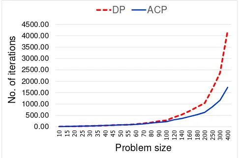
[image:5.595.47.290.71.232.2]DP ACP
Fig. 1. Comparison of the simplex algorithm with DP and ACP.
The sides of problems are varied as shown in table I. For each size, we generate 50 problems and find the mean results for each method.
B. Comparison
To measure the performance of the absolute change pivot rule, we compare this rule with Dantzig’s original pivot rule. The performance measures used for comparison is the number of iterations (pivot). Note that DP is simplex algorithm with Dantzig’s pivot rule and ACP is simplex algorithm with absolute change pivot rule.
Table I shows the comparison between the average number of iterations from solving LP by the simplex algorithm with DP and ACP. This table also shows that the average number of iterations from ACP pivot rule is less than the one from DP. ACP pivot rule achieves less number of iterations when the number of constraints and variable in the problem is higher. Moreover, in figure 1 we found that the number of iteration between ACP and DP is not significantly different in small problem while in large-scale problems ACP have a better performance.
V. SUMMARY OF RESULTS
We proposed a pivot rule called the absolute change pivot rule. The idea of this rule is to have the maximum improvement in the objective value per unit step of the entering variable. We believe that the proposed algorithm could reduce the number of such iteration over the Dantzig’s pivot rule. Table I offers a summary of the average number of iteration of each method. We conclude that the simplex algorithm using the absolute change pivot rule is very fast for solving linear programming problems. Moreover, absolute change pivot rule performs very well on a Klee and Minty problems.
For future works, we may create a new pivot algorithm that have more efficient than absolute change pivot rule and can apply to any linear programming problems.
ACKNOWLEDGMENT
The authors would like to thank the Applied Mathematics and Computational Science Program, Department of
Math-ematics and Computer Science, Faculty of Science, Chula-longkorn University for providing facilities and resources for this research.
REFERENCES
[1] G. B. Dantzig, Linear Programming and Extensions. Princeton: Princeton University Press, 1963.
[2] S. H. Bazara M., Jarvis J.,Linear programming and network flows, 2nd ed. New York: John Whiley, 1990.
[3] V. Klee and G. Minty,How good is the simplex algorithm? in inequal-ities. New York: Academic Press, 1972.
[4] G. D. Forrest J., “A practical steepest-edge simplex algorithm for linear programming,” Mathematical Programming, vol. 57, pp. 341– 374, 1992.
[5] H. P.M.J., “Pivot selection methods of the devex lp code,”Mathematical Programming, vol. 5, pp. 1–28, 1973.
[6] P.-Q. Pan, “A largest-distance pivot rule for the simplex algorithm,”