www.scienceworldjournal.org ISSN 1597-6343
Special Algorithm for the Numerical Solution of System of Initial Value
SPECIAL ALGORITHM FOR THE NUMERICAL SOLUTION OF
SYSTEM OF INITIAL VALUE PROBLEMS FOR ORDINARY
DIFFERENTIAL EQUATIONS USING BLOCK HYBRID EXTENDED
TRAPEZOIDAL RULE OF SECOND KIND
Awari, Y.S1 and M.G. Kumleng2.
1Department of Mathematics/Statistics, Bingham University, Karu. Nigeria 2. Department of Mathematics, University of Jos, Jos. Nigeria
Author’s Correspondence E-mail: [email protected].
ABSTRACT
We develop self-starting family of three and five step continuous extended trapezoidal rule of second kind a block hybrid type (BHETR2s) methods through interpolation and collocation
procedure. The BHETR2s methods are then used to produce
multiple numerical integrators which are each of the same order and assembled into a single block matrix equation. These equations are simultaneously applied to provide the approximate solution for the ordinary differential equations. The stability properties of the methods were investigated and found to be consistent, zero-stable and hence convergent. The block integrators were tested on three numerical initial value problems of ODEs to show accuracy and efficiency.
Keywords: BhETR2s, Zero-Stability, Convergence, General
Linear Method, Collocation Method, Trapezoidal Rule, Ordinary Differential Equation
INTRODUCTION
Ordinary differential equations (ODE’s) are important tools in solving real world problems and a wide variety of natural phenomena are modeled by these ODE’s. Over the years, several researchers have considered the collocation method as a way of generating numerical solutions to ordinary differential equations. The collocation method is dated back as 1956 in the research carried out by Lanczos (1956) and subsequently by Brunner (1996). Lanczos (1956) introduced the standard collocation method with some selected points. However, Fox and Parker (1968) introduced the use of Chebyshev polynomials in collocating the existing method, which was captioned as the Lanczos-Tau method. Ortiz (1969) went on to discuss the general Lanczos-Tau method, which was later extended by Onumanyi and Ortiz (1984) to a method known as the collocation Tau Method. The standard collocation method with method of selected points provides a direct extension of the Tau method to linear ode’s with non polynomial coefficients. The collocation Tau method however, uses the Chebyshev perturbation terms to select the collocation points. Tau-method was extensively studied by Onumanyi and Okunuga (1985, 1986), Okunuga and Sofoluwe (1990). Other researchers such as Fatokun (2007), Onumanyi et al (1994), Adeneyi and Alabi (2006), introduced some other variants of the collocation methods which recently led to some continuous collocation approach.
Collocation methods are widely considered as a way of generating numerical solution to ordinary differential equation of the form:
)
,
(
)
(
y
f
x
y
dx
d
,0 0
)
(
x
y
y
(1)This class of problems arises in the study of (1) is used in simulating the growth of populations, simple harmonic motion, trajectory of a particle etc. With the advent of modern high speed electronic digital computers, the numerical integrators have been successfully applied to study problems in mathematics, engineering, computer science and atmospheric sciences, see Jain et al (2007).
Many numerical integration schemes to generate the numerical solution to problem (1) have been proposed by several authors such as Butcher (2003), Awoyemi et al (2007), Jator (2010) and Akinfenwa (2011). METHODOLOGY: DERIVATION OF THE METHODS
The k-step linear multistep method for the solution of (1) is given in the form
j n k
j j k
j
j n
j
y
h
f
0 0
(2)Which has
k
3
unknowns
j and
j,
j
0
,
1
,...
k
therefore can be of orderk
2
. According to Dahlquist (1963), the order of (2) cannot exceedk
1
(fork
odd) andk
2
(fork
even) for the method to be stable. Authors such as Gear (1965) and Butcher (1980) have proposed modified forms of (2) which were shown to overcome the Dahlquist barrier theorem. These methods known as hybrid methods were obtained by incorporating off-step points in the derivation process.We developed a
k
-step continuous hybrid formula which is an extension of (2) and involvesk
(
x
,
y
)
evaluated at off-grid points (v n v
n
y
x
,
),0
q
k
,
q
0
,
1
,...,
k
in the form:q n q j n k
j j k
j
j n
j
y
h
f
h
f
0 0
(3)
where
k
1
,
0and
0 not both zero,y
nj
y
(
x
jh
)
andf
nv
f
(
x
nv,
y
nv)
, Lambert (1973, 1991). A method such as (3) preserves the traditional advantage of one step methods of being self-starting and permitting easy change of step length, Lambert (1973). Their advantage over R-K methods lies in the fact that they areFu
ll L
en
gt
h Rese
ar
ch
Ar
Special Algorithm for the Numerical Solution of System of Initial Value
less expensive in terms of the number of function evaluation for a given order. The methods also generate simultaneous solutions at all grid points.
The general
k
-step continuous extended trapezoidal rule of second kind, a hybrid type (CHETR2s) with one off-grid collocation point isgiven by: q n q v v j j n j k j j n
j x y h x f h x f
x y
( )
( ) ( ) ) ( 1 1 0
(4)where
j(
x
)
,
j(
x
)
and
v(x
)
are the continuous coefficients of the method,q
is a chosen midpoint of thesubinterval
x
nk1,
x
nk
, Gear (1965). From equation (4), we obtained the D and C matrix as:
1 1 1 1 1 2 1 2 1 1 2 2 2 2 2 2 1 2 1 1 2 2)
2
(
.
.
.
2
1
0
)
2
(
.
.
.
2
1
0
)
2
(
.
.
.
2
1
0
.
.
.
1
.
.
.
.
.
.
.
.
.
.
.
.
.
.
.
.
.
.
.
.
.
.
.
.
1
.
.
.
1
.
.
.
1
k q n q n k v n v n k v n v n k k n k n k n k n n n k n n n k n n nx
k
x
x
k
x
x
k
x
x
x
x
x
x
x
x
x
x
x
x
x
D
(5) and 2 , 2 , 2 , 1 2 , 2 , 1 2 , 2 2 , 2 , 2 , 1 2 , 2 , 1 2 , 2 1 , 1 , 1 , 1 1 , 1 , 1 1 , 2 . . . . . . . . . . . . . . . . . . . . . . . . . . . . . . k q k m k m k v k v k v q m m v v v q m m v v v h h h h h h h h h C
(6)Equations (4), (5) and (6) are therefore used to derived the continuous formulation of the hybrid ETR2s with one off-grid
collocation point for step numbers
k
3
and5
.2.1: Consider
k
3
,
2
5
q
, equation (4) becomes:
2 5 2 5 2 1 2 0
)
(
)
(
)
(
)
(
n j j n j j j nj
x
y
h
x
f
h
x
f
x
y
(7)
From (7), we obtained (5) and (6) as:
4 2 3 2 2 2 2 4 2 5 3 2 5 2 2 5 2 5 4 1 3 1 2 1 1 5 2 4 2 3 2 2 2 2 5 1 4 1 3 1 2 1 1 5 4 3 25
4
3
2
1
0
5
4
3
2
1
0
5
4
3
2
1
0
1
1
1
n n n n n n n n n n n n n n n n n n n n n n n n n n nx
x
x
x
x
x
x
x
x
x
x
x
x
x
x
x
x
x
x
x
x
x
x
x
x
x
x
D
(8) and
6 , 2 6 , 6 , 1 6 , 2 6 , 1 6 , 0 5 , 2 5 , 5 , 1 5 , 2 5 , 1 5 , 0 4 , 2 4 , 4 , 1 4 , 2 4 , 1 4 , 0 3 , 2 3 , 3 , 1 3 , 2 3 , 1 3 , 0 2 , 2 2 , 2 , 1 2 , 2 2 , 1 2 , 0 1 , 2 1 , 1 , 1 1 , 2 1 , 1 1 , 0
h
h
h
h
h
h
h
h
h
h
h
h
h
h
h
h
h
h
C
u u u u u u (9)After some computations, the values of
0(
x
),
1(
x
),
),
(
2
x
1(
x
),
52(
x
)
and
2(
x
)
are obtained from (8)and (9) and substituted into equation (7) to give us the desired continuous formulation for the three step block hybrid ETR2s in
the form:
(10) Equation (10) is evaluated at some
points to obtained discrete equations which we called (11). These equations are combined to form a block, which are implemented to give simultaneously approximate solutions to problem (1).1
4(43𝑦𝑛+3− 141𝑦𝑛+2+ 93𝑦𝑛+1+ 5𝑦𝑛)
=h
2[32𝑓𝑛+5
2
− 39𝑓𝑛+2− 23𝑓𝑛+1]
Special Algorithm for the Numerical Solution of System of Initial Value
1
60(2752𝑦𝑛+5
2
− 2025𝑦𝑛+2− 700𝑦𝑛+1− 27𝑦𝑛) = h
2[16𝑓𝑛+5
2
+ 45𝑓𝑛+2+ 10𝑓𝑛+1]
1
2(1797𝑦𝑛+2− 1704𝑦𝑛+1− 93𝑦𝑛) = h
2[129𝑓𝑛+3−
640𝑓𝑛+5 2
+ 1554𝑓𝑛+2+ 847𝑓𝑛+1]
1
2(−915𝑦𝑛+2+ 480𝑦𝑛+1+ 435𝑦𝑛) = h 2[64𝑓𝑛+5
2
−
465𝑓𝑛+2− 820𝑓𝑛+1− 129𝑓𝑛] (11)
2.2: For
k
5
,
taking2
9
q
, we generate (4) in the form:2 9 2 9 3 1 4 0
)
(
)
(
)
(
)
(
n j j n j j j nj
x
y
h
x
f
h
x
f
x
y
(12)In this case, our D and C matrix becomes:
6 3 5 3 4 3 3 3 2 3 3 6 2 9 5 2 9 4 2 9 3 2 9 2 2 9 2 9 6 2 5 2 4 2 3 2 2 2 2 7 4 6 4 5 4 4 4 3 4 2 4 4 7 3 6 3 5 3 4 3 3 3 2 3 3 7 2 6 2 5 2 4 2 3 2 2 2 2 7 1 6 1 5 1 4 1 3 1 2 1 1 7 6 5 4 3 2 7 6 5 4 3 2 1 0 7 6 5 4 3 2 1 0 7 6 5 4 3 2 1 0 1 1 1 1 1 n n n n n n n n n n n n n n n n n n n n n n n n n n n n n n n n n n n n n n n n n n n n n n n n n n n n n x x x x x x x x x x x x x x x x x x x x x x x x x x x x x x x x x x x x x x x x x x x x x x x x x x x x x D (13) and
8 , 3 8 , 8 , 2 8 , 4 8 , 3 8 , 2 8 , 1 8 , 0 7 , 3 7 , 7 , 2 7 , 4 7 , 3 7 , 2 7 , 1 7 , 0 6 , 3 6 , 6 , 2 6 , 4 6 , 3 6 , 2 6 , 1 6 , 0 5 , 3 5 , 5 , 2 5 , 4 5 , 3 5 , 2 5 , 1 5 , 0 4 , 3 4 , 4 , 2 4 , 4 4 , 3 4 , 2 4 , 1 4 , 0 3 , 3 3 , 3 , 2 3 , 4 3 , 3 3 , 2 3 , 1 3 , 0 2 , 3 2 , 2 , 2 2 , 4 2 , 3 2 , 2 2 , 1 2 , 0 1 , 3 1 , 1 , 2 1 , 4 1 , 3 1 , 2 1 , 1 1 , 0
h
h
h
h
h
h
h
h
h
h
h
h
h
h
h
h
h
h
h
h
h
h
h
h
C
u u u u u u u u (14)The unknown coefficients of the method (12) are obtained after solving D and C matrix where
C
D
1, then substituted back into (12) to yield the CHETR2s for the five step block hybrid ETR2sin the form:
1
24(2193𝑦𝑛+5+ 4545𝑦𝑛+4+ 16640𝑦𝑛+3−
21120𝑦𝑛+2− 2385𝑦𝑛+1+ 127𝑦𝑛= h
2[256𝑓𝑛+9 2⁄ +
1555𝑓𝑛+3− 1059𝑓𝑛+2]
1
2520(748544𝑦𝑛+9 2⁄ − 1488375𝑦𝑛+4− 661500𝑦𝑛+3+
1285956𝑦𝑛+2+ 121500𝑦𝑛+1− 6125𝑦𝑛) =
h
2[128𝑓𝑛+9 2⁄ − 1050𝑓𝑛+3− 567𝑓𝑛+2]
1
24(−166095𝑦𝑛+4− 376540𝑦𝑛+3+ 490320𝑦𝑛+2+
55260𝑦𝑛+1− 2945𝑦𝑛) = h
2[645𝑓𝑛+5− 2816𝑓𝑛+9 2⁄ −
36455𝑓𝑛+3− 24549𝑓𝑛+2] 1
24(−321735𝑦𝑛+4− 108880𝑦𝑛+3+ 397980𝑦𝑛+2+
34320𝑦𝑛+1− 1685𝑦𝑛)=h2[1024𝑓𝑛+9 2⁄ −
10965𝑓𝑛+4− 37640𝑓𝑛+3− 17694𝑓𝑛+2]
1
24(48405𝑦𝑛+4+499100𝑦𝑛+3− 196560𝑦𝑛+2−
342300𝑦𝑛+1− 8645𝑦𝑛) =h2[256𝑓𝑛+9 2⁄ + 23485𝑓𝑛+3+
44919𝑓𝑛+2+ 10965𝑓𝑛+1]
1
8(60885𝑦𝑛+4+ 509520𝑦𝑛+3− 393660𝑦𝑛+2−
222480𝑦𝑛+1+ 45735𝑦𝑛) =h2[1024𝑓𝑛+9 2⁄ + 79320𝑓𝑛+3+
113886𝑓𝑛+2− 3655𝑓𝑛+1] (16)
Stability Analysis
In this paper, we shall discuss the following terminology; order and error constant, consistency and zero-stability of linear multistep methods.
3.1: Order and error constant
Following Fatunla (1991) and Lambert (1973), the local truncation error associated with equation (3) is the linear difference operator ℒ as
ℒ{𝑦(𝑥), ℎ}
k j j n j j nj
y
x
h
y
x
0
)
(
)
(
(17)The Taylor series expansion of (17) about the point
x
nyield ℒ{𝑦(𝑥), ℎ}...
)
(
...
)
(
)
(
1 ( )0
q q nq n
n
c
h
y
x
c
h
y
x
x
y
c
(18)where,
k j jc
00
(19)
k j jj
c
01
(20). . .
k j j q k j j qj
q
j
q
c
0 ) 1 (0
(
1
)!
1
!
1
(21)
where,
q
c
are the constant coefficientsSpecial Algorithm for the Numerical Solution of System of Initial Value
According to Henrici (1962), the method (3) has order
p
if0
...
1
0
c
c
p
c
andc
p1
0
,
wherec
p1iscalled the error constant.
3.2: Consistency
A Linear multistep method (3) is consistent if it has order greater or equal to one (that is
p
1
) that is, if(i)
(
1
)
0
(ii)
(
1
)
(
1
)
where,
and
are the first and second characteristic polynomials of the method.3.3: Zero-Stability
A Linear multistep method (3) is said to be zero stable if no roots of the first characteristic polynomial
(
)
has modulus greater than one and every root with modulus one is distinct, Lambert (1973, 1991).3.4: General Linear Method (GLM)
The GLM were introduced by Burrage and Butcher (1980) and Shirley (2005) on the implementation of LMM for the numerical solution of equation (1).
The GLM for the solution of problem (1) can be expressed in the form
s
j
r
j n j ij n
j j n ij n
i
h
a
f
x
c
h
Y
u
y
i
s
Y
1 1
] [ ]
1 [ ]
1 [
,...,
1
,
)
,
(
(22)
s
j
r
j n j ij n
j i n ij n
i
h
b
f
x
c
h
Y
v
y
i
r
Y
1 1
] [ ]
1 [ ]
1 [
,...,
1
,
)
,
(
(23)N
n
n
0
,
0
,
1
,...,
,h
(
x
ni
x
n)
/
N
andnh
x
x
n
0
andi
1
,
2
,...,
s
are stage values which are internal to each step and represent approximations to the solution at the pointx
n
c
ih
, the vector of external valuesT n r n n n
y
y
y
y
[ ]
[
1[ ],
[2],...,
[ ]]
denotes information available at the end of then
th-step for the input to the next step. Again we emphasize thatr
denotes quantities as output from each step and input to the next step ands
denotes step values used in the computation.These methods are characterized by four matrices
A
,
U
,
B
andV
which make up a partition(
s
r
)
(
s
r
)
matrixM
in the form:
V
B
U
A
M
.
.
.
.
.
(24)
and the general linear method takes the form
1] [
] [
] [
] [
)
(
n n
n n
y
Y
hf
M
y
Y
(25)where,
,
.
.
.
] [
] [ 2 ] [ 1
] [
n s
n n
n
Y
Y
Y
Y
,
)
(
.
.
.
)
(
)
(
)
(
] [
] [ 2 ] [ 1
] [
n s
n n
n
Y
f
Y
f
Y
f
Y
f
] 1 [
] 1 [ 2
] 1 [ 1
] 1 [
.
.
.
n r
n n
n
y
y
y
y
and
] [
] [ 2 ] [ 1
] [
.
.
.
n r
n n
n
y
y
y
y
From (22) to (25), the following definitions hold
Definition 1:
For a GLM (25), the stability matrix
M
(
z
)
is given byU
zA
zB
V
z
M
(
)
(
1
)
1 (26)and the characteristic polynomial given by
))
(
det(
)
,
(
z
I
M
z
(27)Butcher (2003).
Definition 2:
A General Linear Method is A-stable if for all
z
C
1,
I
zA
is non-singular andM
(
z
)
is a stability matrix, Butcher (2003). Note:i. For an A-stable method, there is no restriction on the choice of the step size.
ii. A-stability helps us to determine the type of problems our methods can handle.
Analysis of our Newly Derived Methods
4.1: Three Step Block Hybrid ETR2s (BHETR2s 1)
4.1.1 Order, Consistency and Convergence (BHETR2s 1)
Applying (17) to (21), we obtained the order and error
constant of our method (11) as
p
5
andT
c
)
!
4
23
,
!
5
269
,
)
!
2
(
1
,
!
5
7
(
66
respectively. Since (11)has order
p
5
1
, it is consistent. See (3.1)Special Algorithm for the Numerical Solution of System of Initial Value
4.1.2 Zero-Stability (BHETR2s 1)
The block method (11) can be expressed in the form
(28)
Hence the characteristic polynomial of the block method (11) is given by
(0) (1)
det
)
(
A
A
1 0 0 0
1 0 0 0
1 0 0 0
1 0 0 0
1 0 0 0
0 1 0 0
0 0 1 0
0 0 0 1
det )
(
1
0
)
(
3
1
1
,
2
3
4
0
From (3.3), the method is zero-stable.
4.1.3 GLM for BHETR2s 1
We converted the three step block hybrid ETR2s (11) into GLM
(24) as
(29)
We plotted the absolute stability region of (29) as
Fig. 1: Absolute stability region for BHETR2s 1 method
4.2: Five Step Block Hybrid ETR2s (BHETR2s 2)
4.2.1 Order, Consistency and Convergence (BHETR2s 2)
We obtained the order and error constant of THBH 2 (16) using (17) to
(21) as
p
7
andT
c
)
)
!
2
.(
7
3447
,
)
!
2
(
97
,
)
!
2
.(
7
523
,
)
!
2
.(
7
1217
,
)
!
2
(
45
,
)
!
2
.(
7
13
(
2 8 4 4 4 48
respectively. Since (16) has order
p
7
1
, it is consistent. See (3.1)4.2.2 Zero-Stability (BHETR2s 2)
From (29), the first characteristic polynomial
(
)
of THBH 2(16) is in the form
0
)
1
(
)
det(
)
(
(0)
(1)
5
A
A
, whichimplies that
1
1
and
2
3
4
5
6
0
. Hence, it is zero stable. We have therefore shown the convergence of the method.Special Algorithm for the Numerical Solution of System of Initial Value
4.2.3: GLM for BHETR2s 2
Equation (16) is converted into GLM (24) as
(30)
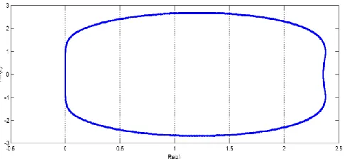
Fig. 2: Absolute stability region for BHETR2s 2 method
Special Algorithm for the Numerical Solution of System of Initial Value
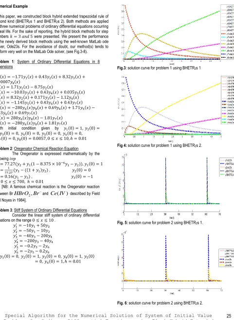
Numerical Example
In this paper, we constructed block hybrid extended trapezoidal rule of second kind (BHETR2s 1 and BHETR2s 2). Both methods are applied
on three numerical problems of ordinary differential equations occurring in real life. For the sake of reporting, the hybrid block methods for step numbers 𝑘 = 3 𝑎𝑛𝑑 5 were presented. We present the performance of the newly derived block methods using the well-known MatLab ode solver, Ode23s. For the avoidance of doubt, our method(s) tends to perform very well on the MatLab Ode solver, (see Fig.3-8).
Problem 1: System of Ordinary Differential Equations in 8 dimensions
𝑦1′(𝑥) = −1.71𝑦1(𝑥) + 0.43𝑦2(𝑥) + 8.32𝑦3(𝑥) +
0.00007𝑦4(𝑥)
𝑦2′(𝑥) = 1.71𝑦1(𝑥) − 8.75𝑦2(𝑥)
𝑦3′(𝑥) = −10.03𝑦3(𝑥) + 0.43𝑦4(𝑥) + 0.035𝑦5(𝑥)
𝑦4′(𝑥) = 8.32𝑦2(𝑥) + 0.171𝑦3(𝑥) − 1.12𝑦4(𝑥)
𝑦5′(𝑥) = −1.145𝑦5(𝑥) + 0.43𝑦6(𝑥) + 0.43𝑦7(𝑥)
𝑦6′(𝑥) = −280𝑦6(𝑥)𝑦8(𝑥) + 0.69𝑦4(𝑥) + 1.71𝑦5(𝑥) −
0.43𝑦6(𝑥) + 0.69𝑦7(𝑥)
𝑦7′(𝑥) = 280𝑦6(𝑥)𝑦8(𝑥) − 1.81𝑦7(𝑥)
𝑦8′(𝑥) = −280𝑦6(𝑥)𝑦8(𝑥) + 1.81𝑦7(𝑥)
with initial condition given by 𝑦1(0) = 1, 𝑦2(0) =
0, 𝑦3(0) = 0, 𝑦4(0) = 0, 𝑦5(0) = 0, 𝑦6(0) = 0,
𝑦7(0) = 0, 𝑦8(0) = 0.0057, 0 ≤ 𝑥 ≤ 10, ℎ = 0.01
Problem 2: Oregenator Chemical Reaction Equation
The Oregenator is expressed mathematically by the following 𝑖𝑣𝑝
𝑦1′ = 77.27(𝑦2+ 𝑦1(1 − 8.375 × 10⁻⁶𝑦1− 𝑦2)), 𝑦1(0) = 1
𝑦2′ = 1
77.27(𝑦3− ((1 + 𝑦1)𝑦2) , 𝑦2(0) = 0
𝑦3′ = 0.16(𝑦1− 𝑦3) , 𝑦3(0) = −1
0 ≤ 𝑥 ≤ 700, ℎ = 0.01
[NB: A famous chemical reaction is the Oregenator reaction between Br
HBrO
2,
Br
andCe
(
IV
)
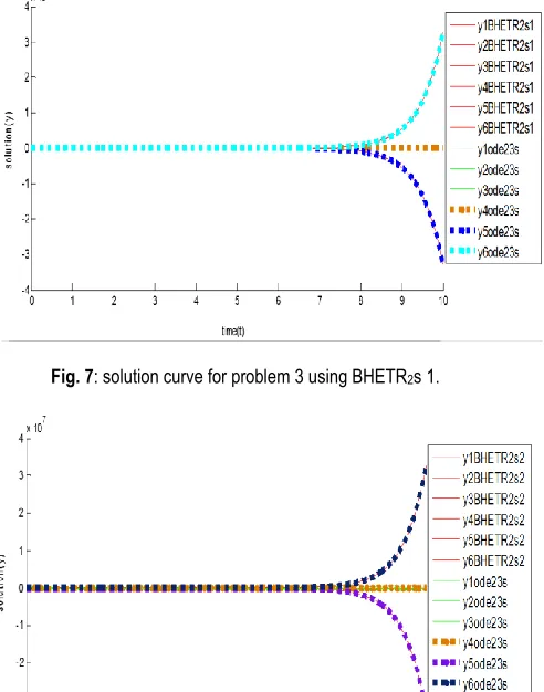
described by Field and Noyes in 1984].Problem 3: Stiff System of Ordinary Differential Equations Consider the linear stiff system of ordinary differential equations on the range 0 ≤ 𝑥 ≤ 10 .
𝑦1′ = −10𝑦1+ 50𝑦2
𝑦2′ = −50𝑦1− 10𝑦2
𝑦3′ = −40𝑦3− 200𝑦4
𝑦4′ = −200𝑦3− 40𝑦4
𝑦5′ = −0.2𝑦5− 2𝑦6
𝑦6′ = −2𝑦5− 0.2𝑦6
𝑦1(0) = 0, 𝑦2(0) = 1, 𝑦3(0) = 0, 𝑦4(0) = 1, 𝑦5(0)
= 0, 𝑦6(0) = 1, ℎ = 0.01
Fig.3: solution curve for problem 1 using BHETR2s 1
Fig 4: solution curve for problem 1 using BHETR2s 2.
Fig. 5: solution curve for problem 2 using BHETR2s 1.
Fig. 6: solution curve for problem 2 using BHETR2s 2.
Special Algorithm for the Numerical Solution of System of Initial Value
Fig. 7: solution curve for problem 3 using BHETR2s 1.
Fig. 8: solution curve for problem 3 using BHETR2s 2.
Conclusion
Our new method(s) competes quite well especially when compared with the Ode Solver. The solution curves show the performance block hybrid methods for step numbers 𝑘 = 3 𝑎𝑛𝑑 5 was quite remarkable especially when compared with the well known 𝑜𝑑𝑒 23𝑠 and 𝑜𝑑𝑒 45. The block hybrid methods were shown to be consistent, zero-stable and hence convergent (see table). Moreover, they were also shown to have order 𝑝 = 𝑘 + 2. Fig.2-8 reveal that our block hybrid methods are A-stable since their region(s) of absolute stability contain the whole of the left hand complex half plane and as such are suitable for the solution of stiff problems.
REFERENCES
Adeniyi, R.B and Alabi, M.O, Derivation of continuous multistep methods using chebyshev polynomials basis functions. Abacus, 33: 351-361
Akinfenwa, O.A., Jator, S.N., Yao,N.M (2011).A linear multistep hybrid methods with continuous coefficient for solving stiff ordinary differential equation.Journal of Modern Mathematics and Statistics 5(2):47-53,2011.
Awoyemi, D.O., Ademiluyi, R.A and Amusegham, E. (2007). Off-grids exploitation in the development of more accurate method for the solution of ODEs, Journal of mathematical
physics, 12 (2007), 117-124
Brugnano, L. and Trigiante, D., Solving Differential Problems by Multistep Initial and Boundary Value Methods, Gordon and Breach Science Publishers, Amsterdam, (1998) Brunner, H., The collocation methods for ODEs: An introduction.
Cambridge University Press.
Butcher, J.C. and Burrage, K. (1980). Non-Linear Stability of a General Class of Differential Equation Methods.BIT, 20: 185-203
Butcher, J.C, Numerical Methods for Ordinary differential systems, John Wiley & sons,west Sussex,England (2003) Dahlquist, G, A special stability problem for linear multistep
methods, BIT,(1963), 3 pp.27-43
Fatokun, J.O. (2007), Continuous approach for deriving self starting Multistep Methods for Initial value problems in ordinary differential equations, Medwell Online J. Eng. Applied Sci. 2(3). 504-508
Fatunla, S.O , Block methods for second order IVP’s. Inter.J.Comp.Maths. 41(1991), pp. 55-63
Fox, L and Parker, I. B. (1968), Chebyshev Polynomials in Numerical Analysis. Oxford University press
Gear, C.W. (1965). Hybrid Methods for Initial Value Problems in Ordinary Differential Systems. SIAM Journal Numerical Analysis. 2: 69-86
Henrici,P., Discrete variable methods for ODE’s. John Wiley, New York ,(1962)
Jain, M.K., Iyengar, S.R and Jain, R.K. Numerical methods for scientific and engineering computation. New Age International (P) Limited Publishers, New Delhi
Jator, S.N. (2010), On the hybrid method with three off-step points for initial value problems. Int. J. Math. Edu. Sci. Technol. 41:110-118
Lambert, J. D , Computational methods for ordinary differential equations, John Wiley, New York, (1973)
Lambert, J. D , Numerical methods for ordinary differential systems. John Wiley, New York ,(1991)
Lanczos, C. (1956), Applied Analysis, New Jersey
Okunuga, S.A and Onumanyi, P. (1985). An accurate collocation method for solving ODEs. AMSE, France, 4(4): 45-48 Okunuga, S.A and Onumanyi, P. (1986). A collocation Tau
method for the solution of ODEs. Abacus, 17: 51-60 Okunuga, S.A and Sofoluwe, A.B (1990). Acollocation method for
non-linear ODEs. AMSE Rev., France, 13(4): 1-6 Onumanyi, P. and Ortiz, E. L (1984). Numerical solution of stiff
and singularly perturbed boundary value problems with a segmented adaptive formulation of the Tau method.
Math. Comput., 43: 189-203
Onumanyi, P., Awoyemi, D.O., Jator, S.N and Sirisena, U.W (1994). New Linear Multistep Methods with continuous coefficients for first order initial value problems. Journal of the Nigeria Mathematical Society 13: 37-51
Ortiz, E.L (1969). The Tau Method. SIAM J. Numerical Analysis, 6: 480-492
Shirley, J.Y. (2005). Implementation of Generalized Linear Multistep Methods for Stiff Differential Equations. Ph.D Thesis (Unpublished), University of Auckland..