1
On a Dual Direct Cosine Simplex Type Algorithm and Its
Computational Behavior
E. M. Badr1 and Khalid Aloufi2
1Scientific Computing Department, Faculty of Computers & Artificial Intelligence, Benha
University, Benha, Egypt. [email protected]
2College of Computer Science & Engineering Taibah University Saudi Arabia
Abstract: The goal of this paper is to propose a dual version of the direct cosine simplex algorithm (DDCA) for general linear problems. Unlike the two-phase and the big-M methods, our technique does not involve artificial variables. Our technique solves the dual Klee-Minty problem in two iterations and solves the dual Clausen’s problem in four iterations. The utility of the proposed method is evident from the extensive computational results on test problems adapted from NETLIB. Preliminary results indicate that this dual direct cosine simplex algorithm (DDCA) reduces the number of iterations of two-phase method.
Keywords: linear programming; dual simplex method; dual direct cosine method; two-phase method.
1. Introduction:
Linear programming is an important cornerstone in the optimization theory. Many realistic problems can be formulated by means of linear mathematical models. The simplex algorithm is the most used tool for solving linear programs. It is an iterative method that was developed by Dantzig [1, 2, 3].
There are many pivot rules for the simplex type algorithm like exterior point simplex algorithm [4, 5, 6] and max-out-in pivot rule [7]. It is known that the application of the simplex algorithm requires at least one basic feasible solution. The two-phase and big-M methods are the most familiar technique for the research of an initial feasible basis. The main drawback of these techniques is requiring the introduction of artificial variables, increasing the dimension of the problem. Wei-Chang Yeh and H.W. Corley [8] proposed a simple direct cosine simplex algorithm (DCA) which solves the Klee-Minty Problem [9] in two iterations and reduced the number of iterations of Simplex
2
in most cases in their computational experiment. In this paper, we propose a dual version of a simple direct cosine simplex algorithm (DDCA) which solves the dual Klee-Minty class of problem in two iterations while the Two phases method solves this class in n+1 iterations where n is the size of the problem. Our technique also solves Clauser class of problems in four iterations but the two phase method solves this class in 2n-1 iterations where n is the size of the problem. Our technique does not require the introduction of artificial variables.
The rest of the paper is organized as follows. Section 2 describes the proposed DDCA algorithm and its characteristics. Benchmark problems “Klee-Minty and Clausen problems” are presented in Section 3. In Section 4, we introduce illustrations of the proposed algorithm with help of two examples. Computational experiments are presented in Section 5, followed by concluding remarks and directions of future research in Section 6.
2. Dual Cosine Simplex Algorithm (DDCA).
We consider the linear programming (LP) problem in standard form:
( )P max b y A y{ T : T c y; 0}, where A is an m n matrix, x and c are
n-dimensional vectors and T denotes transposition. The dual of (P) is the problem
( ) { T : }
D min c x Axb where y is an m-dimensional vector.
For constraint i of (D), define 2 2
cos i ( ij j) / ( ij)
j N j N
a c a
as the cosine of angle ibetween the constraints i and the objective function where bi< 0 and N is the index set
of the non-basic variables.
Remark: The above cosine criterion is only a simple observation without any further proof. Hence, the cosine criterion is not always true.
Dual Cosine Simplex Method (DCSM).
Require: infeasible basis
While bi < 0
Step 1: (Dual feasibility Condition). Let N is the index set of the non-basic variables. The leaving variable ,xi, is the basic variable having the
maximum cosi for minimization problem, where
2 2
cos i ( ij j) / ( ij)
j N j N
a c a
3
the angle between the constraint i and the objective function. If there is a tie, then choose the variable with the most negative value in right hand side.
Step 2: (Dual optimality condition). Given that, xi, is the leaving variable, the
entering variable is the non-basic variable aij < 0 that corresponds to
i ij ij
b
min{| | : a < 0 and j N}
a
The ties are broken arbitrary. If aij0for all non-basic variables then the problem has no feasible solution.
Step3: Apply a pivoting
End while
The current basis is feasible Apply the simplex algorithm.
3. Benchmark problems
In this Section we present two well-known classes of linear programming problems, Klee-Minty class of problems [10] is the first problem and the other is Clausen class of problems [11] as illustrated in the following models:
1
1 1
1
max 10
2 10 100
0, 1, 2,...
n n j
j j
i i j i
j i
j
j
x
subject to x x
x i n
Klee-Minty problem 1 1 1 1 1max (4 / 5)
1
2 (5 / 4) 5
0, 2,...
n j
j j
i i j i
j i
j
j
x
x
subject to x x
x i n
Clausen problemKlee and Minty [10,12] were the first to prove that Simplex has exponential worst-case running time in 1972. An interesting result is that the dual simplex method solves the Klee-Minty problem in a polynomial number of iterations [11]. A more challenging exponential example is given by Clausen [10,11]. The main feature of Clausen’s example is that the primal simplex method is exponential on the primal problem while the dual simplex is exponential on the dual problem.
The following examples show the superiority of our technique over the Two-phase method. Example 1 shows that the two-Two-phase method requires 6 tableaus while our technique requires 3 iterations only, without including the initial one.
4
4.1 Example 1: Consider the following random linear programming problem:
1 2
1 2 1 2 1 2 1 2
1 2
min 4
:
3 3; 3 3; 4 3 6; 2 4
, 0
w x x
subject to
x x x x x x x x
x x
The variables x3, x6 and x4, x5, below are the slack and surplus variables for the
corresponding constraints, respectively. We only need to calculate the corresponding cosiin the Iteration 0 for every i = 1, 2, 3, respectively, as follows:
1
cos # ;
2
2 2 2
[( 3) ( 4) ( 1)( 1)] 169
cos 16.9
( 3) ( 1) 10
2
3 2 2
[( 4) ( 4) ( 3)( 1)] 361
cos 14.44
( 4) ( 3) 25
;
4
cos #
The value of cos2is bigger than that forcos3. We choose x4 as the leaving variable.
From STEP 2, i.e. the entering variable is calculated as follows:
3 3
{| |,| |} 1
3 1
i ij ij
min{| b / a |: a < 0 and jN }
, therefore the element x1 is chosen
as the entering variable. The elementary row operations are the employed to construct a new Simplex Tableau (i.e. STEP 3) as shown in Iteration 1 in Table 3. The entire procedure is repeated until all coefficients in Row 0 are non-positive in Iteration 3 and x3 = 0 , x4 = 2/5, x5 = 9/5 and x6 = 1 are optimal with z = 17/5 in original the problem.
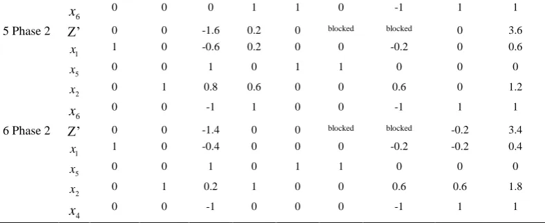
On the other hand, the two-phase method requires 6 tableaus, as shown in Table 2, without including the initial one.
Table 1The Tableau obtained from the proposed DCSM for Example 1.
Iteration
1
x x2 x3 x4 x5 x6 R.H.S
0 Z -4 -1 0 0 0 0 0
3
x 3 1 1 0 0 0 3
4
x -3 -1 0 1 0 0 -3
5
5
6
x 1 2 0 0 0 1 4
1 Z 0 2 0 0 -1 0 6
3
x 0 0 1 1 0 0 0
4
x 1 1/3 0 -1/3 0 0 1
5
x 0 -5/3 0 -4/3 1 0 -2
6
x 0 5/3 0 1/3 0 1 3
2 Z 0 0 0 -8/3 1/5 0 18/5
3
x 0 0 1 1 0 0 0
4
x 1 0 0 -3/5 1/5 0 3/5
5
x 0 1 0 4/5 -3/5 0 6/5
6
x 0 0 0 -1 1 1 1
3 Z 0 0 0 -7/5 0 -1/5 17/5
3
x 0 0 1 1 0 0 0
4
x 1 0 0 -2/5 0 -1/5 2/5
5
x 0 1 0 1/3 0 -3/5 9/5
6
x 0 0 0 -1 1 1 1
Table 2 The Tableau obtained from the Two-Phase Method for Example 1.
Iteration
1
x x2 x3 x4 x5 R1 R2 x6 R.H.S
0 Phase1 Z’ 0 0 0 0 0 -1 -1 0 0
5
x 3 1 0 0 1 0 0 0 3
R1 3 1 -1 0 0 1 0 0 3
R2 4 3 0 -1 0 0 1 0 6
6
x 1 2 0 0 0 0 0 1 4
1 Phase1 Z’ 7 4 -1 -1 0 0 0 0 9
5
x 3 1 0 0 1 0 0 0 3
R1 3 1 -1 0 0 1 0 0 3
R2 4 3 0 -1 0 0 1 0 6
6
x 1 2 0 0 0 0 0 1 4
2 Phase1 Z’ 0 1.67 -1 -1 -2.33 0 0 0 2
1
x 1 0.33 0 0 0.33 0 0 0 1
R1 0 0 -1 0 -1 1 0 0 0
R2 0 1.67 0 -1 -1.33 0 1 0 2
6
x 0 0 0 0 -0.33 0 0 1 3
3 Phase1 Z’ 0 0 -1 0 -1 0 -1 0 0
1
x 1 0 0 0.2 0.6 1 -0.2 0 0.6
R1 0 0 -1 0 -1 0 0 0 0
2
x 0 1 0 -0.6 -0.8 0 0.6 0 1.2
6
x 0 0 0 1 1 0 -1 1 1
4 Phase2 Z’ 0 0 0 0.2 1.6 blocked blocked 0 3.6
1
x 1 0 0 0.2 0.6 0 -0.2 0 0.6
R1 0 0 -1 0 -1 1 0 0 0
2
6 6
x 0 0 0 1 1 0 -1 1 1
5 Phase 2 Z’ 0 0 -1.6 0.2 0 blocked blocked 0 3.6
1
x 1 0 -0.6 0.2 0 0 -0.2 0 0.6
5
x 0 0 1 0 1 1 0 0 0
2
x 0 1 0.8 0.6 0 0 0.6 0 1.2
6
x 0 0 -1 1 0 0 -1 1 1
6 Phase 2 Z’ 0 0 -1.4 0 0 blocked blocked -0.2 3.4
1
x 1 0 -0.4 0 0 0 -0.2 -0.2 0.4
5
x 0 0 1 0 1 1 0 0 0
2
x 0 1 0.2 1 0 0 0.6 0.6 1.8
4
x 0 0 -1 0 0 0 -1 1 1
Example 2: Dual Klee-Minty Problem
Consider the following dual Klee-Minty problem of size n = 3
1 2 3
1 2 3 2 3 3
1 2 3
min 100 10000
:
20 200 100; 20 10; 4 1,
, , 0
w x x x
subject to
x x x x x x
x x x
The variables x4, x5, x6 below are the surplus variables for the corresponding
constraints, respectively. We only need to calculate the corresponding cosiin the Iteration 0 for every i = 1, 2, 3 , respectively., as follows:
2 12
1 2 2 2
[( 1) ( 1) ( 20)( 100) ( 200) ( 10000)] 4.0008 10
cos 99027351.81
( 1) ( 20) ( 200) 40401
2 10
2 2 2 2
[(0) ( 1) ( 1)( 100) ( 20) ( 10000)] 4.004001 10
cos 99850399
(0) ( 1) ( 20) 401
2 8
8
3 2 2 2
[(0) ( 1) (0)( 100) ( 1) ( 10000)] 10
cos 10
(0) (0) ( 1) 1
The value of cos3is bigger than that for cos1 and cos2. We choose x6 as the
leaving variable. From STEP 2, i.e. the entering variable is calculated as follows:
100 100 100 1
{| |,| |,| |}
1 20 200 2
i ij ij
min{| b / a |: a < 0 and jN }
, therefore the
element x3 is chosen as the entering variable. The elementary row operations are the
employed to construct a new Simplex Tableau (i.e. STEP 3) as shown in Iteration 1 in Table 3. The entire procedure is repeated until all coefficients in Row 0 are non-positive in Iteration 1 and x1 = 1 , x2 = x3 = 0 are optimal with z = 104 in original the
7
Table 3 The Tableau obtained from the proposed DCSM for Example 2.
Iteration
1
x x2 x3 x4 x5 x6 R.H.S
0 Z -1 -10 -10000 0 0 0 0
4
x -1 -20 -200 1 0 0 -100
5
x 0 -1 -20 0 1 0 -10
6
x 0 0 (-1) 0 0 1 -1
1 Z -1 -10 0 0 0 -10000 10000
4
x -1 -20 0 1 0 200 100
5
x 0 -1 0 0 1 20 10
3
x 0 0 1 0 0 -1 1
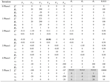
On the other hand, the two-phase method requires 5 tableaus, as shown in Table 4, without including the initial one.
Table 4 The Tableau obtained from the Two-Phase Method for Example 2.
Iteration
1
x x2 x3 x4 x5 x6 R1 R2 R3 R.H.S
0 Phase1 Z’ 0 0 0 0 0 0 -1 -1 -1 0
R1 1 20 200 -1 0 0 1 0 0 100
R2 0 -1 -20 0 -1 0 0 1 0 10
R3 0 0 (-1) 0 0 -1 0 0 1 1
1 Phase1 Z’ 1 21 221 -1 -1 -1 0 0 0 111
R1 1 20 200 -1 0 0 1 0 0 100
R2 0 1 20 0 -1 0 0 1 0 10
R3 0 0 1 0 0 -1 0 0 1 1
2 Phase1 Z’ -0.11 -1.10 0 0.11 -1 -1 -1.11 0 0 0.50
x3 0.01 0.10 1 -0.01 0 0 0.01 0 0 0.50
R2 -0.10 -1 0 (0.10) -1 0 -0.10 1 0 0
R3 -0.01 -0.10 0 0.01 0 -1 -0.01 0 1 0.50
3 Phase1 Z’ 0 -0.05 0 0 0.05 -1 -1 -1.05 0 0.50
x3 0 0.05 1 0 -0.05 0 0 0 0 0.50
x4 -1 -10 0 1 -10 0 -1 10 0 0
R3 0 -0.05 0 0 0.05 -1 0 -0.05 1 0.50
4 Phase1 Z’ 0 0 0 0 0 0 -1 -1 -1 0
x3 0 0 1 0 0 -1 0 0 1 1
x4 -1 -20 0 1 0 -200 -1 0 200 100
R3 0 -1 0 0 1 -20 0 -1 20 10
5 Phase 2 Z’ -1 -100 0 0 0 -104 blocked blocked blocked 10000
x3 0 0 1 0 0 -1 0 0 1 1
x4 -1 -20 0 1 0 -200 -1 0 200 100
x5 0 -1 0 0 1 -20 0 -1 20 10
5. Computational Experiments
8
algorithm (DDCA) with two - phases method. In each test problem, we used different tolerances in order to get the smaller number of iterations with the exact optimum solution. For this comparison, we chose the two phase method [12-15] for the problems contain "" constraints and/or equality constraints.
The programming language used was MATLAB v7.01 SP2 with default options. All codes were run under 64-bit Window 8.1 Operating System having Core(TM)i5 CPU M 460 @2.53GHz, 4.00 GB of memory.
Table 5 The Tableau obtained from the dual cosine, Two-Phases and dual simplex.
Dual Klee-Minty problem Dual Clauser problem
Size Dual cosine
DDCA
Two phase method
Dual cosine DDCA
Two phase method
1 2 1 4 3
2 2 3 4 4
3 2 4 4 5
4 2 5 4 7
5 2 6 4 9
6 2 7 4 11
7 2 8 4 13
8 2 9 4 15
9 2 10 4 17
10 2 11 4 19
From Table 5, the contribution of the proposed algorithm is to solve Klee-Minty problem and Clausen problem with 2 and 4 iterations, respectively, while the simplex method with two phase method spends O(n) iterations for these problems.
Table 6 characterizes 33 NETLIB test problems [16] were used in comparison to test the performance of the algorithms. We transformed the variables ( consist of bounds or are free without limitation) into constraints to keep the algorithms simple. We used LINGO to test the accuracy of the answers obtained using our algorithms.
Table 6 Properties of 33 NETLIB problems
Problem name
Number of onzeros
Density New number of constraints
New number of variables
Number of variables
Number of " " constrains
Number of "" constrains
Number of " = " constrains
adlittle 465 0.0856 56 97 97 40 1 15
afiro 88 0.10185 27 32 32 19 0 8
bandm 2659 0.01847 305 472 472 0 0 305
beaconfd 3476 0.07669 173 262 262 33 0 140
brandy 2150 0.03925 220 249 249 54 0 166
9
fit1d 14,430 0.0134 24 1026 1026 1038 11 1
fit1p 10,894 0.00633 627 1677 1677 399 0 627
grow15 5665 0.00976 300 645 645 600 0 300
grow22 8318 0.00666 440 946 946 880 0 440
grow7 2633 0.02083 140 301 301 280 0 140
kb2 291 0.13649 43 41 41 21 15 16
lotfi 1086 0.02305 153 308 308 42 16 95
recipelp 752 0.0198 91 180 180 77 43 91
sc105 281 0.02598 105 103 103 60 0 45
sc205 552 0.01326 205 203 203 114 0 91
sc50a 131 0.05458 50 48 48 30 0 20
sc50b 119 0.04958 50 48 48 30 0 20
scagr25 2029 0.00862 471 500 500 146 25 300
scagr7 553 0.03062 129 140 140 38 7 84
scfxm1 2612 0.01732 330 457 457 143 0 187
scfxm2 5229 0.00867 660 914 914 286 0 374
scfxm3 7846 0.00578 990 1371 1371 429 0 561
scsd1 3148 0.05379 77 760 760 0 0 77
scsd6 5666 0.02855 147 1350 1350 0 0 147
sctap1 2052 0.01425 300 480 480 0 180 120
share1b 1182 0.0449 117 225 225 28 0 89
share2b 730 0.09626 96 79 79 83 0 13
shell 4900 0.00303 536 1775 1775 119 9 784
ship04l 8450 0.00992 402 2118 2118 40 8 354
ship04s 5810 0.00991 402 1458 1458 40 8 354
stair 3857 0.0186 356 467 467 153 0 698
stocfor1 474 0.0365 117 111 111 48 6 63
Sum 111,017 1.09377 8539 19,531 19,531 5453 454 7079
Average 3364.152 0.03315 258.758 591.849 591.849 165.242 13.7576 214.515
Max 14,430 0.13649 990 2118 2118 1038 180 784
Min 88 0.00303 24 32 32 0 0 1
Tables 6 contains 6 categories of the problems according to the variable numbers range as 30-99, 100-500, 501-999, 1000-1500, 1501-1999 and over 2000 were 6, 15, 5, 4, 2 and 1, respectively. Table 6 contains the largest nonzero number, density, number of variables (after transferring sign constraints), number of constraints (after transferring sign constraints), "" constraint number, "" constraint number, and "=" constraint number.
Table 7 Comparison between the proposed DDCA and two phase method
Problem name
Iterations number Difference in iteration number
Simplex - DCA
DCA Simplex
Phase I
Phase I I
Phase I&II
Phase I
Phase I I
Phase I&II
Phase I
Phase I I
Phase I&II
adlittle 21 99 120 38 100 138 17 1 18
10
bandm 828 323 1151 1042 242 1284 214 -81 133
beaconfd 132 17 149 154 37 191 22 20 42
brandy 731 82 813 521 71 592 -210 -11 -221
etamacro 940 355 1295 944 423 1367 4 68 72
fit1d 52 1664 1716 94 1355 1449 42 -309 -267
fit1p 820 2288 3108 1441 1358 2799 621 -930 -309
grow15 285 205 490 303 485 788 18 280 298
grow22 425 245 670 443 704 1147 18 459 477
grow7 131 78 209 143 168 311 12 90 102
kb2 74 25 99 397 38 435 323 13 336
lotfi 208 164 372 126 77 203 -82 -87 -169
recipelp 300 6 306 299 28 327 -1 22 21
sc105 54 46 100 64 42 106 10 -4 6
sc205 118 110 228 128 115 243 10 5 15
sc50a 24 20 44 29 23 52 5 3 8
sc50b 32 14 46 37 21 58 5 7 12
scagr25 503 869 1372 639 218 857 136 -651 -515
scagr7 126 85 211 159 45 204 33 -40 -7
scfxm1 753 252 1005 802 211 1013 49 -41 8
scfxm2 1592 322 1914 1478 386 1864 -114 64 -50
scfxm3 1947 490 2437 2324 591 2915 377 1 378
scsd1 90 200 290 139 206 345 49 6 55
scsd6 216 184 400 170 447 617 -46 263 217
sctap1 453 161 614 705 163 868 252 2 254
share1b 352 224 576 363 158 521 11 -66 -55
share2b 125 50 175 112 27 139 -13 -23 -36
shell 795 264 1059 843 209 1052 48 -55 -7
ship04l 700 143 843 728 78 806 28 -65 -37
ship04s 488 106 594 499 58 557 11 -48 -37
stair 1019 323 1342 1203 265 1468 184 -58 126
stocfor1 81 12 93 90 29 119 9 17 26
Sum 14421 9433 23854 16467 8385 24852
Average 437 285.848 722.848 499 254.091 753.091
Max 1947 2288 3108 2324 1358 2915
Min 6 6 13 10 7 17
In general, from Table 7, the contribution of the proposed algorithm is that DDCA is generally better than two phase method (22 problems vs. 11 problems). The details of our results as the following:
a) Six problems with the variable numbers 30-99:
DDCA is better than two phase method (5 problems vs. one problem) b) Fifteen problems with the variable numbers 100-500:
11
DDCA is better than two phase method (4 problems vs. one problem) d) Four problems with the variable numbers 1000-1500:
DDCA and two phase methods are equal (2 problems vs. 2 problems) e) Two problems with the variable numbers 1501-1999:
Two phase method is better than DDCA (0 problems vs. 2 problems) f) One problem with the variable numbers over 2000:
Two phase method is better than DDCA (0 problems vs. 1 problem)
6.
Conclusions
We proposed a dual version of the direct cosine simplex algorithm (DDCA) for general linear problems. Unlike the two-phase and the big-M methods, our technique does not involve artificial variables. Our technique solved the dual Klee-Minty problem in two iterations and solved the dual Clausen’s problem in four iterations. The utility of the proposed method is evident from the extensive computational results on test problems adapted from NETLIB. Preliminary results indicate that this dual direct cosine simplex algorithm (DDCA) reduces the number of iterations of two-phase method.
References
[1] G.B. Dantzig, Maximization of a linear function of variables subject to linear inequalities, in: T.C. Koopmans (Ed.), Activity Analysis of production and Allocation, John Wiley, NY, 1951, pp. 339–347.
[2] G.B. Dantzig, Linear Programming and Extensions, Princeton Univ. Press, Princeton, NJ, 1963.
[3] M.S. Bazaraa, J.J. Jarvis, H.D. Sherali, Linear Programming and Network Flows, third ed., John Wiley, NY, 2004.
[4] K. Paparrizos, An exterior point simplex algorithm for general linear problems, Annals of Operation Research 32 (1993) 497–508.
[5] E. S. Badr, K. Paparrizos, N. Samaras, and A. Sifaleras (2005), On the Basis Inverse of the Exterior Point Simplex Algorithm, in Proc. of the 17th National Conference of Hellenic Operational Research Society (HELORS), 16-18 June, Rio, Greece, pp. 677-687.
[6] E.S. Badr, K. Paparrizos, Baloukas Thanasis and G. Varkas (2006), Some computational results on the efficiency of an exterior point algorithm, in Proc. of the 18th National Conference of Hellenic Operational Research Society
12
[7] M. Tipawanna and K. Sinapiromsaran (2013), Max-out-in pivot rule with Dantzig's safeguarding rule for the simplex method, 2nd International Conference on Mathematical Modeling in Physical Sciences
[8] W.-C. Yeh and H.W. Corley, A simple direct cosine simplex algorithm, Applied Mathematics and Computing. 214 (2009) 178–186.
[9] V. Klee, G. Minty, How good is the simplex algorithm?, in: O. Shisha (Ed.), Inequalities–III, Academic Press, NY, 1972, pp. 159–175.
[10] J.Clausen. A tutorial note on the complexity of the simplex algorithm. Technicla Report NR79/16, DIKU, Copenhagen, Denmark, 1979.
[11] K. G. Murty. Linear Programming. John Wiley and Sons, New Yourk, 1983. [12] R. Vanderbei, Linear Programming: Foundations and Extensions, second ed., Kluwer Academic Publishers, Boston, 2001.
[13] P.E.Gill,W.Murray,M.H.Wright,PracticalOptimization,AcademicPress,NY,1981. [14] F.S. Hiller, G.J. Lieberman, Introduction to Operations Research, sixth ed., McGraw-Hill, NY, 1995.
[15] M.S. Bazaraa, J.J. Jarvis, H.D. Sherali, Linear Programming and Network Flows, third ed., John Wiley, NY, 2004.
[16] <http://www.netlib.org/lp/data>.
[17] Elsayed M. Badr, Mahmoud I. Moussa in Wireless Networks (2019), An upper bound of radio k-coloring problem and its integer linear programming model, First Online: 18 March 2019.
[18] Badr, E.;Aloufi,K.A Robot's Response Acceleration Using the Metric Dimension


![Table 6 characterizes 33 NETLIB test problems [16] were used in comparison](https://thumb-us.123doks.com/thumbv2/123dok_us/8013295.1332304/8.595.132.464.254.424/table-characterizes-netlib-test-problems-used-comparison.webp)
