warwick.ac.uk/lib-publications
Manuscript version: Author’s Accepted Manuscript
The version presented in WRAP is the author’s accepted manuscript and may differ from the
published version or Version of Record.
Persistent WRAP URL:
http://wrap.warwick.ac.uk/125362
How to cite:
Please refer to published version for the most recent bibliographic citation information.
If a published version is known of, the repository item page linked to above, will contain
details on accessing it.
Copyright and reuse:
The Warwick Research Archive Portal (WRAP) makes this work by researchers of the
University of Warwick available open access under the following conditions.
Copyright © and all moral rights to the version of the paper presented here belong to the
individual author(s) and/or other copyright owners. To the extent reasonable and
practicable the material made available in WRAP has been checked for eligibility before
being made available.
Copies of full items can be used for personal research or study, educational, or not-for-profit
purposes without prior permission or charge. Provided that the authors, title and full
bibliographic details are credited, a hyperlink and/or URL is given for the original metadata
page and the content is not changed in any way.
Publisher’s statement:
Please refer to the repository item page, publisher’s statement section, for further
information.
Modified Cramér-Rao Bound for
M
-FSK Signal
Parameter Estimation in Cauchy and Gaussian Noise
Junlin Zhang, Nan Zhao,
Senior Member, IEEE
, Mingqian Liu,
Member, IEEE
, Yunfei Chen,
Senior
Member, IEEE
, Hao Song, Fengkui Gong,
Member, IEEE
, and F. Richard Yu,
Fellow, IEEE
Abstract—The Cramér-Rao bound (CRB) provides an efficient standard for evaluating the quality of standard parameter esti-mators. In this paper, a modified Cramér-Rao bounds (MCRB) for modulation parameter estimations ofM-ary frequency-shift-keying (M-FSK) signals is proposed under the condition of the Gaussian and non-Gaussian additive interference. We extend the MCRB to the estimation of a vector of non-random parameters in the presence of nuisance parameters. Moreover, the MCRB is applied to the joint estimation of phase offset, frequency offsets, frequency deviation, and symbol period ofM-FSK signal with two important special cases of alpha stable distributions, namely, the Cauchy and the Gaussian. The extensive simulation studies are conducted to contrast the MCRB for the modulation parameter vector in different noise environments.
Index Terms—Modified Cramér-Rao bound, parameter esti-mation, frequency-shift-keying, impulsive noise.
I. INTRODUCTION
C
OGNITIVE radio (CR) is a promising technology forperformance enhancement in vehicular networks, which allows the combination of artificial intelligence and software-defined radios. A major challenge of CR is the accurate en-vironmental awareness and blind parameter estimations at CR receivers, which is a key feature for promoting efficient and secure communications in the CR context [1]. The Cramér-Rao bound (CRB) is the fundamental lower bound on the variance of any unbiased estimator, which has been proven that the optimal performance of any parameter estimator can be achieved [2]. However, when the observed signal con-tains modulated data, carrying out the statistical expectations
This work was supported by the National Natural Science Foundation of China under Grant 61501348, 61801363 and 61871065, Shaanxi Provincial Key Research and Development Program under Grant 2019GY-043, Joint Fund of Ministry of Education of the People’s Republic of China under Grant 6141A02022338, China Postdoctoral Science Foundation under Grant 2017M611912, the 111 Project under Grant B08038 and the China Scholarship Council under Grant 201806965031.(Corresponding author: Mingqian Liu.)
J. Zhang, M. Liu and F. Gong are with the State Key Laboratory of Inte-grated Service Networks, Xidian University, Shaanxi, Xi’an 710071, China (e-mail: [email protected]; [email protected]; [email protected]).
N. Zhao is with the School of Information Science and Technology, Qingdao University of Science and Technology, Qingdao, 266000, P. R. China, and also with the School of Information and Communication Engineering, Dalian University of Technology, Dalian 116024, P. R. China. (email: [email protected]).
Y. Chen is with the School of Engineering, University of Warwick, Coventry, West Midlands United Kingdom of Great Britain and Northern Ireland CV4 7AL (e-mail: [email protected])
H. Song is with Wireless@VT, Department of ECE, Virginia Tech, Blacks-burg, VA, 24061, USA (e-mail: [email protected]).
F. R. Yu is with the Department of System and Computer Engineering, Carleton University, Ottawa, Ontario Canada K1S 5B6, Canada (e-mail: [email protected]).
involved in evaluating the CRB is extremely challenging. To avoid the high computational complexity caused by the unwanted parameters, a modified CRB (MCRB) is proposed as a better alternative [3].
Analytical MCRB for parameter estimations has been wide-ly studied in several literatures, such as active and passive localization [4], blind demodulations [5], and channel iden-tification [6]. Unfortunately, the methods introduced in these literatures rely on a strong assumption of the additive white Gaussian noise (AWGN) channel. Many experimental studies have shown that radio channels may experience non-Gaussian noise, such as the symmetric alpha stable (SαS) distribution. For example, non-Gaussian noise occurs in low frequency communications [7] and shallow underwater acoustic com-munications [8]. In [9], G. Yang et al. derived the CRB for joint timing and carrier phase offsets estimations of minimum shift keying signals in alpha-stable noise. In [10], M. Liu et al. investigated the CRB on the accuracy of estimating the direction-of-arrival parameter in impulsive noise. In [11], Y. Chen et al. provided the CRB of frequency estimations for complex sinusoid signals in symmetric alpha stable noise. To the best of our knowledge, the MCRB enabled joint parameter estimations forM-ary frequency-shift-keying (M-FSK) signals in Cauchy and Gaussian noise have not been studied.
Therefore, the MCRB used for parameter estimations is derived for M-FSK signals in Cauchy and Gaussian noise. To be specific, we propose an analytical method to derive expressions of the MCRB for joint estimations of phase offset, frequency offsets, frequency deviation, and symbol period of M-FSK signal in Cauchy and Gaussian noise. The contributions of this paper can be summarized as two aspects. First, we extend the MCRB to the joint estimation of a vector of non-random parameters in the presence of random nuisance parameters under Cauchy and Gaussian noise. Second, we derive the MCRB for a parameter vector from M-FSK signal over fading channels in Cauchy noise.
II. SYSTEMMODEL
The continuous-time baseband equivalent of FSK signal with phase and frequency offsets can be given by
s(t) =Aejθej2πfct∑
le
j2πf∆slth(t−lT
b), (1)
sl∈ {˜sm|˜sm= 2m−1−M, m= 1,· · ·, M}.
Assume that the signal is corrupted by additive noise. The received signal can be expressed as
r(t) =s(t) +w(t) , (2)
where s(t) represents a complex baseband FSK signal, and
w(t)is additive noise. When the signal is affected by fading channel and is corrupted by additive noise, the received signal can be derived by
rη(t) =sη(t) +w(t), (3)
wheresη(t)represents the FSK signal over fading channel
sη(t) =Aejθej2πfct ∑
lηle
j2πf∆slth(t−lT
b). (4)
whereηlis non-constant fading gain.
The noise w(t) is a random variable following the sym-metric alpha-stable (SαS) distribution. The SαS distribution is defined by its characteristic function as
φ(ω) = exp (jδω−γ|ω|α), (5)
where α is the characteristic exponent, δ is the location parameter, andγis the dispersion of the distribution. A stable distribution is called standard if δ = 0 and γ = 1. The alpha stable distribution has no closed-form expression for the probability density function (PDF) except for two important special cases, namely, the Cauchy (α= 1), and the Gaussian (α= 2). The Cauchy distribution is given by
f1(γ, δ;x) =
1 π
γ
γ2+ (x−δ)2. (6)
Besides, the Gaussian distribution is given by
f2(γ, δ;x) =
1
√πγexp
(
−(x−δ) 2
γ
)
. (7)
The mixed signal to noise ratio (MSNR) is employed to describe the signal and noise power ratio in this paper.
MSNR = 10log10 (
σs2/γ), (8)
whereσ2
sis the signal variance, andγis dispersion coefficient of the alpha stable noise.
III. MCRBFORM-FSK PARAMETERESTIMATION
A. MCRB in Cauchy Noise
To jointly estimate a parameter vector of λ =
(θ, fc, f∆, Tb)T, we assume that a vectorλwith finite dimen-sional can be uesed to representr(t)with adequate accuracy in the observed interval. The PDF of the received signalr(t), with the Cauchy distribution noise can be expressed as
ρ(r|s,λ) =∏L
l=1(2π) −1
γ
(
γ2+|rl−sl|
2)−3/2
, (9)
whereLis the observation time ands=∆{sl}is the vector of transmitted symbols. The log-likelihood function is
lnρ(r|s,λ) =Llog (γ)−Llog (2π)
−1.5∑L
l=1log (
γ2+|rl−sl|
2)
, (10)
c ∆ b 1 4
a vector parameter to be estimated. For any parameter
λm(m= 1,· · · ,4), the fundamental lower bound on the error variance is given as
Er
[(
ˆ λm−λm
)2]
≥MCRBλ(λm) = [
Ic−1(λ) ]
m,m. (11)
[Ic(λ)]m,n=Er
[
−∂2lnρ(r|s,λ)
∂λm∂λn ]
, (12)
where Ic(λ) is Fisher Information Matrix (FIM), [·]m,n represents the element of the matrix at row m and column
n, andEr[·]denotes statistical expectation with respect to the subscripted variable r. First, we calculate the derivatives of the log likelihood function given in (10) with respect to the components ofλas follows.
∂lnρ(r|s, λ) ∂λm
=− ∂
(
1.5
L ∑ t=1
log
(
γ2+|x(t)−s(t)|2))
∂λm
=−3
L ∑
t=1
|w(t)| γ2+|w(t)|2
∂s(t) λm
.
(13)
Then, by using (13), allows us to compute the [Ic(λ,s)]m,n as follows.
[Ic(λ,s)]m,n=E {
∂2lnρ(r|s, λ)
∂λm∂λn }
= 9E
{L ∑
t=1
|w(t)| γ2+|w(t)|2
∂s∗(t) ∂λm
L ∑
t=1
|w(t)| γ2+|w(t)|2
∂s(t) ∂λn
}
= 9E
L ∑
t=1
|w(t)|2
(
γ2+|w(t)|2)2
∂s∗(t)∂s(t) ∂λm∂λn
= 3 5γ2
∫
Es [
Re
(
∂s∗(t)∂s(t) ∂λm∂λn
)]
dt,
(14)
where E
{
|w(t)|2
(γ2+|w(t)|2)
}
= 15γ22. In order to determine
the expression of [Ic(λ,s)]m,n, we should go through
Es [
Re
(
∂s∗(t)∂s(t)
∂λm∂λn
)]
(m=n) which can be written as fol-lows
Es
[ ∂s(t)∂θ
2]
=A2Es
[∑L l=1h
2(t−lT
b) ]
, (15)
Es
[ ∂s(t)∂fc
2]
= 4π2A2t2Es
[∑L l=1h
2(t−lT
b) ]
, (16)
Es
[ ∂s(t)∂f∆
2]
= 4π2A2t2Es
[∑L l=1s
2 lh
2(t−lT
b) ]
, (17)
Es
[ ∂s(t)∂Tb
2]
=A2Es
[∑L l=1l
2h˙2(t−lT
b) ]
, (18)
where h(t˙ −Tb) is the derivative of h(t−Tb) with respect to Tb. Denote Λ = 3A2/(5γ2), C = E
s[sls∗l], ℑ1 = ∫
Tb
∑L l=1h
2(t−lT
b)dt,ℑ2= ∫
Tbt
∑L l=1h
2(t−lT
b)dt,ℑ3= ∫
Tbt
2∑L
l=1h
2(t−lT
b)dt,Ω = ∫
T0
∑L l=1l
2h˙2(t−lT
According to (14)-(18), the elements of I(λ, s) are ex-pressed as
[Ic(λ,s)]1,1= Λℑ1, (19)
[Ic(λ,s)]2,2= 4π
2Λℑ
3, (20)
[Ic(λ,s)]3,3= 4π
2ΛCℑ
3, (21)
[Ic(λ,s)]4,4= ΛΩ. (22)
Using the same procedure, we can derive the
Es [
Re
(
∂s∗(t)∂s(t)
∂λm∂λn
)]
(m̸=n)as follows
Es
[
Re
(
∂s∗(t) ∂θ
∂s(t) ∂fc
)]
=2πtA2Es
[∑L l=1h
2(t−lT
b) ]
, (23)
Es
[
Re
(
∂s∗(t) ∂θ
∂s(t) ∂f∆
)]
=2πtA2Es
[∑L l=1slh
2(t−lT
b) ]
, (24)
Es
[
Re
(
∂s∗(t) ∂fc
∂s(t) ∂f∆
)]
=(2πtA)2Es
[∑L l=1slh
2(t−lT
b) ]
, (25)
Es
[
Re
(
∂s∗(t) ∂θ
∂s(t) ∂Tb
)]
=Es
[
Re
(
∂s∗(t) ∂fc ·
∂s(t) ∂Tb
)]
=Es
[
Re
(
∂s∗(t) ∂f∆ ·
∂s(t) ∂Tb
)]
= 0.
(26)
Substituting (23)-(26) into (14), the elements of Ic(λ,s) for m̸=nare expressed as
[Ic(λ,s)]1,2= [Ic(λ,s)]2,1= 2πΛℑ2, (27)
[Ic(λ,s)]1,3= [Ic(λ,s)]3,1= 2πΛBℑ2, (28)
[Ic(λ,s)]2,3= [Ic(λ,s)]3,2= 4π
2ΛBℑ
3, (29)
[Ic(λ,s)]1,4= [Ic(λ,s)]4,1= 0, (30)
[Ic(λ,s)]2,4= [Ic(λ,s)]4,2= 0, (31)
[Ic(λ,s)]3,4= [Ic(λ,s)]4,3= 0. (32)
where B = Es[sl]. According to (19)-(22) and (27)-(32),
Ic(λ,s)can be written as
Ic(λ,s)=
Λℑ1 2πΛℑ2 2πΛBℑ2
2πΛℑ2 4π2Λℑ3 4π2ΛBℑ3
2πΛBℑ2 4π2ΛBℑ3 4π2ΛCℑ3
ΛΩ
. (33)
Substituting (33) in (11), the MCRBs for λ =
(θ, fc, f∆, Tb)T can be derived as
MCRBcλ(θ) =ℑ3/(Λ (ℑ1ℑ3− ℑ2ℑ2)), (34)
MCRBcλ(fc) =
Cℑ1ℑ3−B2ℑ2ℑ2
4π2Λℑ
3(ℑ1ℑ3− ℑ2ℑ2)
, (35)
MCRBcλ(f∆) = 1 /(
4π2Λℑ3 (
C−B2)), (36)
MCRBcλ(Tb) = 1/(ΛΩ). (37)
Using a similar approach, we derive the FIM Ic(µ,s) for parameter vector ofµ= (θ, fc, f∆)
T
which can be given as
Ic(µ,s) =
2πΛΛℑℑ12 4πΛ2π2Λℑℑ23 4π2πΛB2ΛBℑℑ23
2πΛBℑ2 4π2ΛBℑ3 4π2ΛCℑ3 . (38)
Substituting (38) in (11), the MCRBs forµ= (θ, fc, f∆) T
can be expressed as
MCRBcµ(θ) =ℑ3/(Λ (ℑ1ℑ3− ℑ2ℑ2)), (39)
MCRBcµ(fc) = (
Cℑ1ℑ3−B2ℑ2ℑ2 )
4π2Λℑ
3(ℑ1ℑ3− ℑ2ℑ2)
, (40)
MCRBcµ(f∆) = 1 /(
4π2Λℑ3 (
C−B2)). (41)
For the parameter vector of υ = (θ, fc) T
, we can obtain
Ic(υ,s)by using the same procedure.
Ic(υ,s) = [
Λℑ1 2πΛℑ2
2πΛℑ2 4π2Λℑ3 ]
. (42)
Substituting (42) in (11), the MCRBs forυ = (θ, fc) T
are expressed as
MCRBcυ(θ) =ℑ3/(Λ (ℑ1ℑ3− ℑ2ℑ2)), (43)
MCRBcυ(fc) =ℑ1 /(
4π2Λ (ℑ1ℑ3− ℑ2ℑ2) )
. (44)
For the parameter vector ofσ= (θ, f∆)T,Ic(σ,s)can be expressed as
Ic(σ,s) = [
Λℑ1 2πΛBℑ2
2πΛBℑ2 4π2ΛCℑ3 ]
. (45)
Substituting (45) in (11), the MCRBs for the parameter set
σ= (θ, f∆)T, are written as
MCRBcσ(θ) =Cℑ3 /(
Λ(Cℑ1ℑ3−B2ℑ2ℑ2 ))
, (46)
MCRBcσ(f∆) =ℑ1 /(
4π2Λ(Cℑ1ℑ3−B2ℑ2ℑ2 ))
. (47)
For the parameter vector ofν= (fc, f∆) T
, we can express
Ic(ν,s)as
Ic(ν,s) = [
4π2Λℑ
3 4π2ΛBℑ3
4π2ΛBℑ
3 4π2ΛCℑ3
]
. (48)
Substituting (48) in (11), the MCRBs for the parameter set
ν= (fc, f∆) T
written as
MCRBcν(fc) =C /
4π2Λℑ3 (
C−B2), (49)
MCRBcν(f∆) = 1 /(
4π2Λℑ3 (
C−B2)). (50)
B. MCRB in Gaussian Noise
Considering an observation vectorr= (r1, r2,· · ·, rL) T
in Gaussian noise, the PDF of the received signal r(t) can be expressed as
p(r|s,λ) = √1 πexp
( −1
γ
∫
|rl−sl| 2
dt
)
, (51)
where s =∆ {sl} is the vector of transmitted symbols. The log-likelihood function becomes
lnp(r|s,λ) =−1 γ
∫
|rl−sl| 2
dt. (52)
For any parameter λm(m= 1,· · · ,4), the fundamental lower bound on the error variance given as
Er
[(
ˆ λm−λm
)2]
≥MCRBλ(λm) = [
Ig−1(λ) ]
[Ig(λ)]m,n=Er −
∂λm∂λn
, (54)
where,Ig(·)is FIM,[·]m,n represents the factor of the matrix with row m and column n, and Er[·] denotes statistical expectation with respect to the subscripted variable r. This gives
[Ig(λ,s)]m,n=
2 γ
∫
Es
[
Re
(
∂s∗(t) ∂λm ·
∂s(t) ∂λn
)]
dt. (55)
Similar to Section A, we can obtain the following equations
[Ig(λ,s)]1,1=ℜℑ1, (56)
[Ig(λ,s)]2,2= 4π2ℜℑ3, (57)
[Ig(λ,s)]3,3= 4π2ℜCℑ3 (58)
[Ig(λ,s)]4,4=ℜΩ, (59)
[Ig(λ,s)]1,2= [J(λ, s)]2,1= 2πℜℑ2, (60)
[Ig(λ,s)]1,3= [J(λ, s)]3,1= 2πℜBℑ2, (61)
[Ig(λ,s)]2,3= [J(λ, s)]3,2= 4π
2ℜBℑ
3, (62)
[Ig(λ,s)]1,4= [J(λ, s)]4,1= 0, (63)
[Ig(λ,s)]2,4= [J(λ, s)]4,2= 0, (64)
[Ig(λ,s)]3,4= [J(λ, s)]4,3= 0. (65)
where ℜ = 2A2/γ. Using (56)-(65), the FIM Jg(λ,s) is given by
Ig(λ,s) =
ℜℑ1 2πℜℑ2 2πℜBℑ2
2πℜℑ2 4π2ℜℑ3 4π2ℜBℑ3
2πℜBℑ2 4π2ℜBℑ3 4π2ℜCℑ3 ℜΩ
. (66)
Substituting (66) in (53), the MCRBs for λ =
(θ, fc, f∆, Tb) T
written as
MCRBgλ(θ) =ℑ3/(ℜ(ℑ1ℑ3− ℑ2ℑ2)), (67)
MCRBgλ(fc) = (
Cℑ1ℑ3−B2ℑ2ℑ2 )
4π2ℜℑ
3(ℑ1ℑ3− ℑ2ℑ2)
, (68)
MCRBgλ(f∆) = 1 /(
4π2ℜℑ3 (
C−B2)), (69)
MCRBgλ(Tb) = 1/(ℜΩ). (70)
For the parameter vector of µ= (θ, fc, f∆)T, we can also obtain the MCRBs
MCRBgµ(θ) =ℑ3/(ℜ(ℑ1ℑ3− ℑ2ℑ2)), (71)
MCRBgµ(fc) = (
Cℑ1ℑ3−B2ℑ2ℑ2 )
4π2ℜℑ
3(ℑ1ℑ3− ℑ2ℑ2)
, (72)
MCRBgµ(f∆) = 1 /(
4π2ℜℑ3 (
C−B2)), (73)
For the parameter vector of υ = (θ, fc)T, the MCRBs given by
MCRBgυ(θ) =ℑ3/(ℜ(ℑ1ℑ3− ℑ2ℑ2)), (74)
MCRBgυ(fc) =ℑ1 /(
4π2ℜ(ℑ1ℑ3− ℑ2ℑ2) )
. (75)
∆ as
MCRBgσ(θ) =Cℑ3 /(
ℜ(Cℑ1ℑ3−B2ℑ2ℑ2 ))
, (76)
MCRBgσ(f∆) =ℑ1 /(
4π2ℜ(Cℑ1ℑ3−B2ℑ2ℑ2 ))
, (77)
For the parameter vector of ν = (fc, f∆) T
, the MCRBs expressed as
MCRBgν(fc) =C /(
4π2ℜℑ3 (
C−B2)), (78)
MCRBgν(f∆) = 1 /(
4π2ℜℑ3 (
C−B2)). (79)
C. MCRB for Fading Channel with Cauchy Noise
In this section we consider the MCRB for modulation parameter estimations of FSK signals over the fading channel with Cauchy noise. Since the noisew(t)is Cauchy noise, the PDF of the received signalr(t)can be expressed as
ρ(rη|sη,λ) = ∏L
l=1(2π) −1
γ
(
γ2+rlη−slη2
)−3/2
,
(80) where sη
∆
= {sl η
}
is the vector of transmitted symbols is affected by fading channel. The log-likelihood function is
lnρ(rη|sη,λ) =Llog (γ)−Llog (2π)
−1.5∑L
l=1log (
γ2+rηl −slη2
)
, (81)
Let λ = (θ, fc, f∆, Tb)T = (λ1, . . . , λ4)T be the modula-tion parameter vector. Based on (11) and (12), this bound on the variance of any unbiased estimate is given by
Er
[(
ˆ λm−λm
)2]
≥MCRBλ(λm) = [
Iη−1(λ,sη) ]
m,n. (82)
[Iη(λ,sη)]m,n=Er
[
−∂2lnρ(rη|sη,λ)
∂λm∂λn ]
, (83)
where [Iη(λ,sη)]m,n is Fisher Information Matrix (FIM). Using the same procedure in section A, [Iη(λ,s)]m,n can be written as
[Iη(λ,sη)]m,n=
3 5γ2
∫
Es
[
Re
(∂s∗ η(t)
∂ρm
·∂sη(t)
∂ρn )]
dt. (84)
Similarly,Es
[
Re
(∂s∗
η(t)
∂ρm ·
∂sη(t)
∂ρn
)]
can be written as follows
Es
[ ∂s∂θη(t)
2
]
=A2Es
[∑L l=1η
2 lh
2(t−lT
b) ]
, (85)
Es
[ ∂s∂fη(t)c
2]
= 4π2A2t2Es
[∑L l=1η
2 lh
2(t−lT
b) ]
, (86)
Es
[ ∂s∂fη(t)∆
2]
= 4π2A2t2Es
[∑L l=1s
2 lη
2 lh
2(t−lT
b) ]
, (87)
Es
[ ∂s(t)∂Tb
2]
=A2Es
[∑L l=1η
2 ll
2h˙2(t−lT
b) ]
. (88)
Es
[
Re
(
∂s∗η(t)
∂θ
∂sη(t)
∂fc )]
=A(t) 2πtEs
[∑L l=1η
2 lh
2(t−lT
b) ]
Es
[
Re
(
∂s∗η(t)
∂θ
∂sη(t)
∂f∆ )]
=A(t) 2πtEs
[∑L l=1slη
2 lh
2(t−lT
b) ]
, (90)
Es
[
Re
(
∂s∗(t) ∂fc
∂s(t) ∂f∆
)]
=A(t)Es
[∑L l=1slη
2 lh
2
(t−lTb) ]
, (91)
Es
[
Re
(∂s∗ η(t)
∂θ
∂sη(t)
∂Tb )]
=Es
[
Re
(∂s∗ η(t)
∂fc
·∂sη(t)
∂Tb )]
=Es
[
Re
(∂s∗ η(t)
∂f∆ ·
∂sη(t)
∂Tb )]
= 0.
(92)
where A(t) = (2πtA)2. We assumed that,
Λ = 6A2/(5γ2), Υ1 = ∫
Tb
∑L l=1η
2 lh
2(t−lT
b)dt,
Υ2 =
∫ Tbt
∑L l=1η
2 lh
2(t−lT
b)dt, Υ3 =
∫ Tbt
2∑L
l=1ηl2h2(t−lTb)dt,Ψ = ∫
T0
∑L
l=1l2ηl2h˙2(t−lTb)dt. The elements of Iη(λ, s)are expressed as
[Iη(λ,sη)]1,1= ΛΥ1, (93)
[Iη(λ,sη)]2,2= 4π2ΛΥ3, (94)
[Iη(λ,sη)]3,3= 4π2ΛCΥ3, (95)
[Iη(λ,sη)]4,4= ΛΨ. (96)
[Iη(λ,sη)]1,2= [Iη(λ,s)]2,1= 2πΛΥ2, (97)
[Iη(λ,sη)]1,3= [Iη(λ,s)]3,1= 2πΛBΥ2, (98)
[Iη(λ,sη)]2,3= [Iη(λ,s)]3,2= 4π2ΛBΥ3, (99)
[Iη(λ,sη)]1,4= [Iη(λ,s)]4,1= 0, (100)
[Iη(λ,sη)]2,4= [Iη(λ,s)]4,2= 0, (101)
[Iη(λ,sη)]3,4= [Iη(λ,s)]4,3= 0. (102)
According to (93)-(102), Iη(λ,sη)can be written as
Iη(λ,sη)=
ΛΥ1 2πΛΥ2 2πΛBΥ2
2πΛΥ2 4π2ΛΥ3 4π2ΛBΥ3
2πΛBΥ2 4π2ΛBΥ3 4π2ΛCΥ3
ΛΨ
. (103)
Application of (103) to (82) yields,
MCRBηλ(θ) = Υ3/(Λ (Υ1Υ3−Υ2Υ2)), (104)
MCRBηλ(fc) =
CΥ1Υ3−B2Υ2Υ2
4π2ΛΥ
3(Υ1Υ3−Υ2Υ2)
, (105)
MCRBηλ(f∆) = 1 /(
4π2ΛΥ3 (
C−B2)), (106)
MCRBηλ(Tb) = 1/(ΛΨ). (107)
Similarly, for the parameter vector of µ= (θ, fc, f∆) T
, the MCRBs can be expressed as
MCRBηµ(θ) = Υ3/(Λ (Υ1Υ3−Υ2Υ2)), (108)
MCRBηµ(fc) = (
CΥ1Υ3−B2Υ2Υ2 )
4π2ΛΥ
3(Υ1Υ3−Υ2Υ2)
, (109)
MCRBηµ(f∆) = 1 /(
4π2ΛΥ3 (
C−B2)). (110)
For the parameter vector of υ= (θ, fc)T, we can also obtain the MCRBs as follow,
MCRBηυ(θ) = Υ3/(Λ (Υ1Υ3−Υ2Υ2)), (111)
MCRBηυ(fc) = Υ1 /(
4π2Λ (Υ1Υ3−Υ2Υ2) )
. (112)
For the parameter vector of σ = (θ, f∆) T
, the MCRBs are written as
MCRBησ(θ) =CΥ3 /(
Λ(CΥ1Υ3−B2Υ2Υ2 ))
, (113)
MCRBησ(f∆) = Υ1 /(
4π2Λ(CΥ1Υ3−B2Υ2Υ2 ))
. (114)
For the parameter vector of ν = (fc, f∆) T
, we can express the MCRBs as
MCRBην(fc) =C /
4π2ΛΥ3 (
C−B2), (115)
MCRBην(f∆) = 1 /(
4π2ΛΥ3 (
C−B2)). (116)
We can make the following remarks concerning the de-scribed derivation.
Remark 1: The MCRBs of the parameter vector λ are
dependent on the amplitude A and dispersion coefficient γ
in Cauchy and Gaussian noise. When MSNR is given, the MCRBs with Gaussian noise is less than MCRBs with Cauchy noise.
Remark 2: For the parameter vector of λ, MCRBs for
modulation parameter estimation of M-FSK signal are de-pendent on the amplitudeA, dispersion coefficientγ, shaping functionh(t)and observation timeL. In addition, MCRBs for frequency offsetsfc and frequency deviation f∆ are affected by data symbols{sl}.
Remark 3: For the case of M-FSK modulated sequence
transmitted over fading channel, the fading gain is one of important factor affecting MCRBs. In other words, the worse the fading channel, the higher the MCRBs.
IV. NUMERICALRESULTS
In this section, the numerical simulation results of the derived MCRBs are presented followed with the corresponding analysis. In simulations, the signal amplitude A is unity, the symbol time Tb is normalized to unity, the carrier frequency
fc is set to 10/Tb, the carrier phase θ is set arbitrarily between 0 and2π, the frequency deviationf∆ is set to2/Tb. The observation time is 100 so that there are 100 symbols available for estimations. The parameters of the Cauchy noise (α = 1) and Gaussian noise (α = 2) are selected as a location parameterδ= 0 and a dispersion coefficientγ = 1. The consider a fading channel is modeled as an independent Rayleigh flat fading channel.
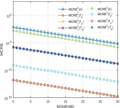
Fig.1 and Fig.2 demonstrate the MCRBs of the joint estimation parameter vector λ = (θ, fc, f∆, Tb)
T
MSNR(dB)
0 5 10 15 20 25 30
MCRB
10-15 10-10 10-5 100
MCRBCλ(θ)
MCRBC
λ(fc)
MCRBCλ(f∆)
MCRBC
λ(Tb)
MCRBC(θ)
MCRBC(fc) MCRBC(f
∆)
MCRBC(T
[image:7.612.334.529.64.243.2]b)
Fig. 1. MCRB of joint estimation and individual estimation for M-FSK signals in Cauchy noise
MSNR(dB)
0 5 10 15 20 25 30
MCRB
10-15 10-10 10-5 100
MCRBCλ(θ)
MCRBC
λ(fc)
MCRBC
λ(f∆)
MCRBC
λ(Tb)
MCRBC(θ) MCRBC(f
c)
MCRBC(f∆) MCRBC(Tb)
Fig. 2. MCRB of joint estimation and individual estimation for M-FSK signals in Gaussian noise
with Gaussian noise is less than MCRBs with Cauchy noise for given amplitude A.
In Fig. 3, we evaluate the MCRBs of the joint estimation parameter vector λ= (θ, fc, f∆, Tb)
T
and the MCRBs of the individual estimation parameter when FSK modulated signal is affected by fading channel and is corrupted by additive Cauchy noise. From the figure, we note that the MCRBs with joint estimations are also higher than MCRBs with individual estimations for the carrier phasesθ and carrier frequency fc. Moreover, comparing Fig.3 and Fig.1, we can find out that the MCRBs for modulation parameter estimations from FSK signals over fading channel are all less than MCRBs with Cauchy noise for given MSNR, indicating that the worse the fading channel, the higher the MCRBs.
V. CONCLUSION
This paper has derived the MCRB to estimate the mod-ulation parameters of M-FSK signals in Cauchy noise and
MSNR(dB)
0 5 10 15 20 25 30
MCRB
10-15 10-10 10-5 100
MCRBCλ(θ)
MCRBC
λ(fc)
MCRBCλ(f∆)
MCRBC
λ(Tb)
MCRBC(θ) MCRBC(f
c)
MCRBC(f
∆)
MCRBC(T
[image:7.612.72.269.65.243.2]b)
Fig. 3. MCRB of joint estimation and individual estimation for M-FSK signals over Fading channel
Gaussian noise. The modulation parameters considered are the frequency offsets, carrier phases, frequency deviation and symbol duration. In addition, we investigated the MCRB for a parameter vector λ from M-FSK signal over fading channels in Cauchy noise. Theoretical analysis and simulations demonstrated that the smaller the characteristic exponentαof the noise, the higher the MCRBs for given MSNR. And the worse the fading channel, the higher the MCRBs for given MSNR. The MCRB approach seems to be applicable in many other modulation types, such as PSK and QAM .
REFERENCES
[1] S. Majhi and T. Ho, "Blind symbol-rate estimation and test bed imple-mentation of linearly modulated signals," IEEE Trans. Veh. Technol., vol. 64, no. 3, pp. 954-963, Jun. 2014.
[2] Y. Yang, Hua Peng, and D. Zhang, "Modified Cramér-Rao bound of parameter estimation for single-channel mixtures of adjacent-frequency signals,"IET Signal Process., vol. 10, no. 9, pp. 1082-1088, Dec. 2016. [3] F. Gini, R. Reggiannini, and U. Mengali, "The modified Cramér-Rao bound in vector parameter estimation,"IEEE Trans. Commun., vol. 46, no. 1, pp. 52 - 60, Jan. 1998.
[4] L. Gui, M. Yang, H. Yu, J. Li, F. Shu, and F. Xiao, "A Cramér-Rao lower bound of CSI-based indoor localization,"IEEE Trans. Veh. Technol., vol. 67, no. 3, pp. 2814-2818, Mar. 2018.
[5] J. P. Delmas, "Closed-form expressions of the exact Cramér-Rao bound for parameter estimation of BPSK, MSK, or QPSK waveforms,"IEEE Signal Process. Lett., vol. 15, pp. 405-408, Jun. 2008.
[6] Y. Li, H. Minn, and J. Zeng, "An average Cramér-Rao bound for frequency offset estimation in frequency-selective fading channels,"
IEEE Trans. Wireless Commun., vol. 9, no. 3, pp. 871 - 875, Mar. 2010. [7] G. Yang, J. Wang, G. Zhang, and S. Li, "Communication signal pre-processing in impulsive noise: a bandpass myriad filtering-based method,"IEEE Commun. Lett., vol. 22, no. 7, pp. 1402-1405, Jul. 2018. [8] G. Zhang, J. Wang, G. Yang, Q. Shao, and S. Li, "Nonlinear processing for correlation detection in symmetric alpha-stable noise,"IEEE Com-mun. Lett., vol. 25, no. 1, pp. 120-124, Jan. 2018.
[9] G. Yang, J. Wang, G. Zhang, Q. Shao, and S. Li, "Joint estimation of timing and carrier phase offsets for MSK signals in alpha-stable noise,"
IEEE Commun. Lett., vol. 22, no. 1, pp. 89-92, Jan. 2018.
[10] M. Liu, J. Zhang, J. Tang, F. Jiang, P. Liu, F. Gong, N. Zhao. "2-D DOA robust estimation of echo signals based on multiple satellites passive radar in the presence of alpha stable distribution noise,"IEEE Access, vol. 7, pp. 16032-16042, Nov. 2019.
[image:7.612.71.268.298.475.2]