Classical Analysis over Credit Allotment Scheme using
Classification under Machine Learning Domain
Satyam S. Sundaram
M.Tech (CSE) Scholar
MIET, Meerut
Pradeep Pant
Professor (CSE)
MIET, Meerut
ABSTRACT
As the amount of data is increasing over the tremendous rate, it is extremely viable to imply smart analysis. It deals with optimization of performance criterion dealing with examples relevant to present and past situations. Learning plays a vital role in making predictions from analysis of data set properties. Amongst the various applications in the domain of learning we have a training data set over which learning is implied as the data that is collected may contain irrelevant features that are avoidable in our process and also do not contribute towards learning .We also ensure that the selected data set suits our purpose of predicting futuristic events and unseen samples. However while dealing with problems of classification in machine learning we need to determine and draw observations relevant to a problem statement having disjoint set of training data. Mining information from data enrolls classification, clustering and other such methodologies as its subsets. The paper presents a classical descriptive procedure to compare various classification schemes under single roof and draw analysis over the best scorer in terms of accuracy to draw predictions of credit allotment to customer problem. Various data sets can be filtered by the approached schemes to make decision during binary and multi valued classification. However the paper ranks one over other to determine the best fit choice in terms of performance measures.
Keywords
Learning, Features, Classification
1.
INTRODUCTION
Having being evolved from the study of pattern recognition in artificial intelligence, Machine learning proliferates the study of algorithms that acquires properties of learning and making predictions from the analyzed data set. The range of problems employed in learning are diverse therefore templates of classification are applied appropriate to classification scheme. In domain of learning come supervised and unsupervised learning theories. The field of data analytics bases its floor on the frontiers of unsupervised learning paradigms. However the growing importance roots its reason from the factors that the data sets are too complex for humans to sense with understanding and these algorithms employed in learning can improve transparency of analysis.
This field threads itself with mathematical parameters and methods of probability and statistics to establish correlation between the visualized data and make inferences for it. However overruling statistics which concentrates on asymptotic analysis it generally focuses on bounds. The current paper focuses itself on prediction of credit scoring which is highly viable due to severe market competition. However mining important information from available training data set it is imputable to apply artificial intelligence and use classification as central strategy to predict scores whether credit must allotted to customer who apply for a loan
or not. Data mining usually deals with extraction of important informed buried in data to discover underlying trends and patterns.
The problem of credit scoring has gained great attention as this industry roots its benefits from risk reduction, insuring policies and focusing on market strategies. Usually credit scoring is applied to rank credit information and to target collection activities including application form details and the information held by a credit reference agency on the applicant [2]. As a result accounts having high default rate can be monitored and necessary actions can be taken to minimize risk factors. In this direction statistical, non parametric statistical methods and artificial intelligence approaches have been proposed to support credit approval decision process [3][4]. We can categorize a credit score as bad or good to predict whether or not it will be allotted to a customer based on the details input in the model adopted for classification. Our objective is to stimulate the system and ensure best result in terms of machine performance with our focus on attaining accuracy.
1.1
Learning as a Subject
In context of machine learning we usually focuses on three learning paradigms:
1.1.1. Supervised Learning
:In this type of learning we establish correspondence between feature set and labeled set which imbibes knowledge from the properties of data set under consideration. In our technique we base our results on classification methodology as a subset of supervised learning paradigm where each feature set corresponds to definite class label. This knowledge will help in prediction and recognition [1] illustrated in Fig 1.
1.1.2. Unsupervised Learning:
When there is no comprehension over the available data set and we apply probabilistic techniques to associate features together broadly known as clustering then unsupervised learning springs to action.
1.1.3. Reinforcement Learning:
Fig 1: Supervised Learning
2. PARADIGMS OF CLASSIFICATIONS
As the problem of learning is quite extensive; various templates have been designed for it2.1 Binary Classifications
It assumes a given pattern say a from domain A and associate a value with it in the form of random variable say b {+-1}, whatever it will assume. It is applied in various aspects like we judge whether an email received is a spam or not, whether a given fruit is apple or orange. The Fig 2 shows an explicit explanation of the given classification where the pattern of circles is differentiated from that of distribution of square in a 2 class problem.
2.2
Multiclass Classification
[image:2.595.53.281.73.224.2]It is a logical extension of binary classification where the random variable b assumes range of values from 1 to n. The main difference lies in the error introduced during estimation. For instance the problem of assessing breast cancer which may be mistaken as healthy status for a patient who is in early stages of development and may be misinterpreted in latter stages where it is incurable. Fig 3 shows the model of multiclass classification which can be termed as regression where value are not limited to strict classification, instead we have a range of predicted result values.
Fig 2: Binary Classification Fig 3: Multiclass Classification
2.3 Structure Estimation
It assumes that other than the values used by b, it is ensured that b is associated with some structural parameters for advance results.
2.4
Novelty Detection
[image:2.595.322.526.390.526.2]It focuses on unusual observations regarding past parameter estimation. The choice of unusual prediction is a subjective issue and moreover these occasions occur less frequently. So the task is to assign a novel value to each observation to explicit the occurrence of events. A simple example can illustrate the concept where scores of each character describe its novelty as shown in Fig 4.
Fig 4: Novelty Detection
3.
MODELS OF CLASSIFICATION
A classification generally assigns a class label to data set under consideration. With multiplicity or variety in information set as a problem presented to the machine it is imperiable for it to investigate the relevant class or category for future analysis. The choice of model influences the accuracy parameter during evaluation of results. Variety of classification algorithms are proposed to achieve class label under machine learning paradigm:3.1
Decision Tree Analysis
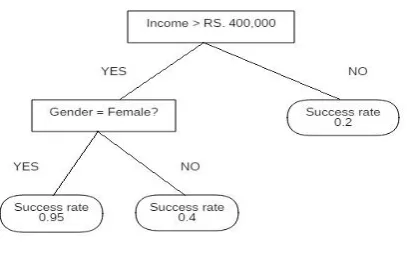
The algorithm for decision tree finds its applications both in classification as well as regression problems. It generally works by portioning of input space into corresponding regions each having its data values as elements of complete data set as shown in Fig 5.
Fig 5: Decision Tree
Under the family of supervised machine learning algorithms its prime requirements are to predict the class or category by developing a training model by utilization of machine learning rules based on prior data inferences or results obtained from training data sets. It builds a tree representation to depict the problem solution where the attributes are illustrated by means of internal nodes and leaves are assigned with label we are looking for. To select the appropriate attributes that make up the root node is quite challenging. Proper selection needs to be carried out to ensure accuracy else results are catastrophically poor. Various methods like Gini index and information gain facilitate the selection of attributes by estimation of information content in that attribute. With the attributes that carry huge information the selection is favored for the same. It is likely based upon a rule based system.
3.2 Random Forest
[image:2.595.65.257.488.612.2]well as regression problems. In random forest we generally select features to build the nodes amongst the subset of randomly available features to promote diversity in applying it over range of data values. It generally prevails over decision tree in calculating the importance of each feature after training so that the sum of all features selected turns up to 1. However feature selected while building trees in random forest is an important parameter of discussion as more the no of features greater are the chances of over fitting. It generally builds smaller tress from the feature subset available and reduces the problem of over fitting to a great extent. The various parameters used in random forest do increase the predictive power of the model so ensure accuracy and computational speed with which it determines the results
(a) Firstly the concept of m estimators are taken in consideration which ensures that more the no of tress in forest higher is the performance of model while predicting result but at the same time suffers from drawback in managing the computational; speed of the model.
(b) To overcome the computational speed problem is to determine the randomness of the model which tends to give same results with training sets repeatedly tested.
So with these hyper parameters efficiency improves but prediction on real time data remains the bottleneck of the model.
3.2
Support Vector Machine
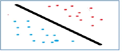
Support vector machine is another algorithm of relevance widely employed in classification problems. In the training process the model generally analyze the available data as input and predicts patterns embedded in the data in a hyper plane which is multi dimensional feature space. All the input patterns are represented by points on this feature space which are then mapped to the output categories in a way that these categories are clearly divisible by a gap as far as possible. However to best explain the concept of SVM, maximal margin classifier is employed. With two input variables projected on a two dimensional space the hyper plane is chosen in a way that it separates those variables best in two classes either 0 or 1 in case of binary classification problems.
[image:3.595.317.527.72.172.2]As an example if we are provided with two balls data set one which is blue colored and other red, the linear classifier separates two classes of objects in the manner shown in Fig 6:
Fig 6: classification by linear classifier
[image:3.595.318.534.241.343.2]But with the growing complexity of data sets it is imperiable to employ SVM that best deals with such problems as depicted in the fig 7:
Fig 7: classification by SVM
Instead of creating complex curves the non separable problems are solved using kernel concept where objects on left hand side as shown in fig 8 are rearranged using kernel functions to look separable with a simple hyper plane illustration.
Fig 8: Solving non separable problems by kernel implementation
3.3
Logistic Regression
Another algorithm that is widely employed in classification to measure the relationship between categorical and independent variables through probability calculation using logistic function. However the algorithm does not fit with problems of regression where output is continuous valued. It can be employed to give accurate result in problems where the output is either binary as in our problem set to predict whether a customer will be allotted credit from bank or not or in examples where the scores of student in various subjects are utilized to predict whether he/she will get admitted in a university or not.
3.4
Neural Networks
Neural network technique has been inspired from the working of biological neurons wherein a computer is programmed to learn inferences from observational data. It finds its application in areas of image, pattern recognition and suitably used for classification problems. It consists of multiple layers where learning and analysis is facilitated. The network learns by adjusting weight parameters between layers connected to each other in order to process data and ensure correct predictions.
4.
PROBLEM STATEMENT
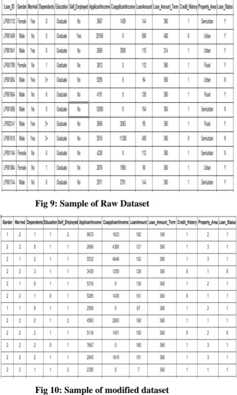
[image:3.595.54.262.546.636.2]Fig 9: Sample of Raw Dataset
Fig 10: Sample of modified dataset
5.
PERFORMANCE MEASURES
Following factors are considered for measuring the
correctness of classification algorithm.5.1
Confusion Matrix
Confusion matrix or error matrix summarizes the performance of classification. This matrix is of 2 * 2 in case of binary classification. Columns refer to the predicted class while rows refer to the actual class. For values are the outcomes of confusion matrix.
True Positive (TP): Actual positive is also predicted positive.
True Negative (TN): Actual negative is also predicted negative.
False Positive (FP): Predicted positive but actual value is negative.
False Negative (FN): Predicted negative but actual value is positive.
Fig 11: Confusion Matrix Structure
5.2
True Positive Rate (TPR)
TPR is also called Sensitivity or Recall. It measures the number of positives correctly classified out of the total positives in the test data. TPR is the number of True Positives divided by the sum of True Positives and False Negatives.
TPR / Sensitivity / Recall = TP / (TP + FN)
5.3
False Positive Rate (FPR)
FPR, also called fall-out, is the number of False Positives divided by the sum of False Positives and True Negatives. It measures the number of negatives incorrectly classified out of the total negatives in the test data.
FPR = FP / (FP + TN)
5.4
Specificity
Specificity is also True Negative Rate (TNR). It is the number of True Negatives divided by the sum of True Negatives and False Positives. Specificity refers to the ability of classifying the negative results.
Specificity / TNR = TN / (TN + FP)
5.5
Precision
Precision is the Positive Predicted Value. It is the number of True Positives divided by the sum of True Positives and False Positives. It measures the exactness of classifier in predicting the positives.
Precision = TP / TP + FP
5.6
AUC
AUC refers to the area under the ROC curve. ROC is Receiver Operating Characteristics. ROC is a plot of True Positive Rate against the False Positive Rate. The diagonal of the ROC chart is representing the trivial classifier which assigns the class randomly. If ROC tends to bend towards the upper left corner of the chart then classification can be termed as good classification. The model having the highest ROC curve is termed as the best model for classification.
5.7
Error Rate (ER)
Error rate is the number of misclassifications divided by the total number of examples in the testing dataset. The value of error rate varies from 0 to 1. The lower value is more desirable as we need lesser misclassifications. It is calculated as
ER = (FN + FP) / N = (FN + FP) / (TP + TN + FN + FP)
5.8
Accuracy
Accuracy of a classifier refers to the number of correct classification made out of the total classifications made by a classifier. What percentage of test data is correctly predicted is measured by the accuracy.
Accuracy = (TP + TN) / (TP + FP + TN + FN)
5.9
F Score
F Score is also a measure of the accuracy of classifier. It takes into account the balance between the Precision and Recall. It is the harmonic mean of Recall and Precision.
5.10
Youden’s Index
Youden’s Index measures a classification model by using sensitivity and specificity. It is the arithmetic mean of sensitivity and specificity.
Youden’s Index = Sensitivity - (1 - Specificity)
5.11
Matthews Correlation Coefficient
(MCC)
MCC is a measure of quality of a classifier. It takes into account all the outcomes of confusion matrix. MCC can be used in case of different size classes also. MCC is the correlation coefficient between the actual and the predicted. Its value varies from -1 to 1 where +1 represents perfect classification, 0 refers to no better than random classification and -1 represent the low correspondence between the actual and the predicted.
MCC = (TP * TN – FP * FN) / SQRT ((TP + FP) * (TP + FN) * (TN + FP) * (TN + FN))
6.
STIMULATION RESULT
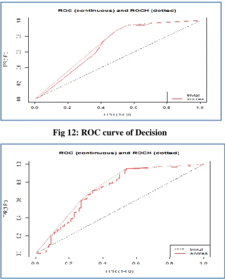
[image:5.595.315.548.73.639.2]The above problem statement when implemented in R language forecast the results in the form of ROC curve & many different parameters. ROC curves for considered algorithms are shown in Fig 12, Fig 13, Fig 14, Fig 15 and Fig 16. The results of other performance measures as mentioned in the above part are shown in Fig 17 & Fig 18 for all considered models. From the ROC curve it is inferred that that when the considered classification algorithms are applied on the training datasets, the AUC value of curve is maximum with SVM implementation. But on the basis of evaluating testing data with performance measures as shown in Fig 18 different parameters infer that accuracy of model relies strongly upon random forest in a general manner .Therefore credit allotment data sets works well when random forest algorithm are applied to predict future results.
Fig 12: ROC curve of Decision
Fig 13: ROC curve of linear classification
Fig 14: ROC curve of Random forest
Fig 15: ROC curve of SVM
[image:5.595.54.285.456.743.2]Fig 17: Values of Confusion Matrix for different models
Fig 18: Performance Measures of different models
7.
COMPARISON CHART OF
DIFFERENT MODELS
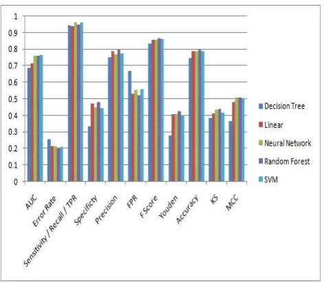
[image:6.595.57.295.249.455.2]The comparison between different models after simulation in R language is represented in the Fig 19. The chart has parameters on x-axis and corresponding values on y-axis which ranges from 0 to 1. This chart shows that Random Forest model wins over SVM in parameter count like error rate, accuracy, FPR etc. From this comparison chart it is clear that though the AUC value for random forest and SVM are likely to be same but in other performance parameter the Random Forest outweighs the SVM model. On basis of Accuracy, F Score, Youden’s Statistic & MCC coefficient the Random Forest model performs better in comparison of all other models for the loan allocation problem.
Fig 19: Comparison chart of performance measures for different models
8.
CONCLUSION
In this paper the algorithm or model that is best suitable to predict accuracy during credit allotment by banks to customer have been studied and verified by means of diverse algorithms from which Random Forest is inferred to be the best. Various problem of multiclass classification will be covered in future works to compare and analyze the efficiency of models over each other and generate new models from the drawbacks of existing system.
9.
REFERENCES
[1] http://disp.ee.ntu.edu.tw/~pujols/Machine%20Learning% 20Tutorial.pdf
[2] http://cmapspublic3.ihmc.us/rid=1MSXWCGGP-1C6ZQFT-14FT/Lee_CART_MARS.pdf
[3] Chen, M.S., Han, J.,Yu, P.S.”Data mining: an overview from a database perspective”. IEEE Trans. Knowledge Data Eng. Vol,8,1993
[4] Cheng, B., Titterington, D.M, “Neural network: a review from a statistical perspective “Statist. Sci.,Vol.9,1994.
[5] K. Huang, H. Yang, I. King, and M. R. Lyu, ``Local learning vs. global learning: An introduction to maxi-min margin machine,'' in Support Vector Machines: Theory and Applications. Berlin, Germany: Springer, 2005, pp. 113_131.
[6] E. E. Elattar, J. Goulermas, and Q. H. Wu, ``Electric load forecasting based on locally weighted support vector regression,'' IEEE Trans. Syst., Man, Cybern. C, Appl. Rev., vol. 40, no. 4, pp. 438_447, Jul. 2010.
[7] K. Grolinger, M. A. M. Capretz, and L. Seewald, ``Energy consumption prediction with big data: Balancing prediction accuracy and computational resources,'' in Proc. IEEE Int. Congr. Big Data (BigData Congress), Jun. 2016, pp. 157_164.
41 [9] W. Watanabe. Pattern recognition: Human and
mechanical. Wiley, 1985.
[10] E. Yom-Tov. An introduction to pattern classification. In U. von Luxburg, O. Bousquet, and G. R¨atsch, editors, Advanced Lectures on Machine Learning, volume 3176 of LNAI, pages1–23. Springer, 2004.
[11] L. Yang, Y. Chu, J. Zhang, L. Xia, Z. Wang, and K.-L. Tan, ``Transfer learning over big data,'' in Proc. 10th Int. Conf. Digit. Inf. Man- age. (ICDIM), Oct. 2015, pp. 63_68.
[12] S. Thrun and L. Pratt, Learning to Learn. Norwell, MA: Kluwer, 1998. D. L. Silver, Q. Yang, and L. Li, ``Lifelong machine learning systems: Beyond learning algorithms,'' in Proc. AAAI Spring Symp., 2013, pp. 49_55.
[13] M. T. Khan, M. Durrani, S. Khalid, and F. Aziz, ``Lifelong aspect extraction from big data: Knowledge engineering,'' Complex Adapt. Syst. Model., vol. 4, no. 1, pp. 1_15, 2016.
[14] Z. Chen and B. Liu, ``Topic modeling using topics from many domains, lifelong learning and big data,'' in Proc. 31st Int. Conf. Mach. Learn., 2014, pp. 703_711. [15] S. Suthaharan, ``Big data classi_cation: Problems and
challenges in network intrusion prediction with machine
learning,'' ACM SIGMETRICS Perform. Eval. Rev., vol. 41, no. 4, pp. 70_73, 2014.
[16] T. Dietterich, ``Ensemble methods in machine learning,'' in Multiple Classi_er Systems, vol. 1857. London, U.K.: Springer-Verlag, 2000,pp 1.15
[17] Jerome Friedman, Trevor Hastie, Robert Tibshirani, “Additive Logistic Regression: A statistical view of Boosting”, The Annals of Statistics 2000, Vol 28, No.2, 337-407.
[18] (2000)Gradient boosting. On Wikipedia the free
encyclopedia. Available:
http://en.wikipedia.org/wiki/Gradient_boosting
[19] Shotaro Matsumoto, Hiroya Takamura, and Manabu Okumura “Sentiment Classification Using Word Sub-sequences and Dependency Sub-trees” Advances in Knowledge Discovery and Data Mining ,301-311, 9th Pacific-Asia Conference, PAKDD 2005, Hanoi, Vietnam, May 18-20, 2005. Proceedings