J. Phys. A: Math. Gen.36(2003) 3379–3383 PII: S0305-4470(03)54067-7
Saddle points in the chaotic analytic function and
Ginibre characteristic polynomial
M R Dennis and J H Hannay
H H Wills Physics Laboratory, Tyndall Avenue, Bristol BS8 1TL, UK Received 27 September 2002, in final form 10 December 2002 Published 12 March 2003
Online atstacks.iop.org/JPhysA/36/3379
Abstract
Comparison is made between the distribution of saddle points in the chaotic analytic function and in the characteristic polynomials of the Ginibre ensemble. Realizing the logarithmic derivative of these infinite polynomials as the electric field of a distribution of Coulombic charges at the zeros, a simple mean-field electrostatic argument shows that the density of saddles minus zeros falls off as
π−1|z|−4from the origin. This behaviour is expected to be general for finite or
infinite polynomials with zeros uniformly randomly distributed in the complex plane, and which repel.
PACS numbers: 05.45.Mt, 02.10.Yn, 02.30.Sa
It is well known that there are several similarities between the distributions of zeros of the ensemble of random polynomials which tend to the chaotic analytic function (discussed by Hannay 1996, 1998, Bleheret al 2000, Forrester and Honner 1999, Leboeuf 1999,
Bogomolnyet al1996) and the eigenvalues of Ginibre matrices (Ginibre 1965,Mehta 1991, ch 15), both in the finite and infinite cases. To be more precise, forNlarge and possibly∞, we compare the zeros of the chaotic analytic function polynomials (caf polynomials)
fN ,caf(z)= N
n=0
anzn
√
n! (1)
where the an are independent identically distributed complex circular Gaussian random
variables, with the eigenvalues of matrices in the Ginibre ensemble, defined to beN ×N
matrices with entries independent identically distributed complex circular Gaussian random variables. The Ginibre analogue to equation (1) is the characteristic polynomialfN ,Gin(z).
The zeros of the twofN share the following properties, as discussed in the above references:
• they are uniformly randomly distributed, with densityσ =1/π, within a disc centred on the origin of the complex plane, which has radius√N, and smoothed boundary (Ginibre with Gaussian tail outside, caf with power law);
• within this disc, the distribution of zeros is statistically invariant to translation and rotation; • the statistical properties of the zeros at a fixed radiusrdo not change asNincreases,
provided that√N r+O(1);
• the two-point correlation functionsgcaf, gGinfor zeros separated by distance|z1−z2| =
r√N−O(1)within the disc are given by
gcaf(
√
2r)=[(sinh2r2+r4)coshr2−2r2sinhr2]/sinh3r2 (2)
gGin(r)=1−exp(−r2). (3)
Both of these functions exhibit quadratic repulsion at the origin, are of order 1 (uncorrelated) forr 1 and satisfy a screening relation: the integral of σ g over the plane, after subtracting the uniform background density, is−1;
• the distribution of Ginibre zeros is equivalent to a two-dimensionalN-charge Coulomb gas in a harmonic oscillator potential|z|2/2, at a temperature corresponding toβ = 2,
whereas the caf zeros have an additionalN-body potential.
Despite these similarities, there is no obvious explicit relation between these two ensembles. In this work, we consider the distribution of the saddle points of the polynomialsfcaf, fGin
(dropping the suffixNunless necessary), that is zeros of the derivative df/dz. The behaviour of the caf saddles is easy to determine; the Ginibre saddles less so. Numerical experiment shows that in both cases the saddle distribution roughly mimics the zero distribution, except for a surplus near the origin and a deficit near the disc edge. Using the electrostatic analogy, we shall see that the density of the saddles minus zeros has the same 1/π|z|4tail away from the origin for each case, due to the repulsion of the zeros. Also, the cause and extent of the edge deficit will be clear.
The density of caf saddlesρcan be found by replacingfcafwithfcaf in the formula for
the density of zeros (Hannay 1996,Nonnenmacher and Voros 1998, equation (69)). When |z|√N−O(1), theN → ∞formulae may be applied. In this case, the zero densityσ is 1/π(as mentioned above), and the saddle density is
ρ=π−1∂z∂z∗lnfcaf (z)fcaf (z)∗ →π−1(1 +(1 +|z|2)−2). (4)
This has, in addition to a uniform 1/πdensity, a ‘bump’ in the vicinity of the origin, which integrates to 1, and the saddle surplus isρ−σ =(π(1 +|z|2)2)−1, which decays likeπ−1|z|−4.
For finiteN, of course, an orderNpolynomial hasN−1 saddles, notN + 1, implying that
ρ ≈ 0 for|z|2 N −2, which is indeed the case when the calculation in equation (4) is
performed for finiteN. The pattern of zeros and saddles for a sample caf polynomial with
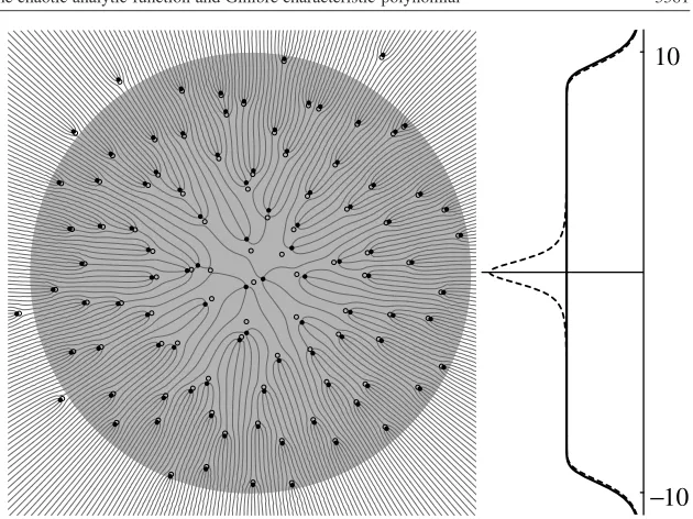
N =100 is shown in figure1(the pattern of Ginibre zeros and saddles looks very similar), along with the corresponding plots ofσ andρ; the most obvious feature of this distribution is that zeros and saddles tend to occur in ‘bonded’ pairs, with the saddle positioned radially inwards from the zero, and the bond length decreases as|z|increases. The pairing breaks down near the origin, indeed the ‘extra’ unbonded zero is in this neighbourhood.
It proves to be more convenient to work with the cumulative number of saddles minus zeros within a radiusr= |z|, denoted byN(r), which is given by
N(r)=2π
r
0
(ρ−σ )rdr (5)
≈1−1/r2 for caf,with 1 r√N−O(1). (6) It is our aim to show, using mean-field electrostatics, that this expression holds generally for polynomials with zeros distributed according to the bullet points above, including the Ginibre polynomialsfGin. Figure2shows numerical plots ofN(r)for simulations of both the caf and
−
10
10
Figure 1. A sample distribution of zeros and saddles for a caf polynomial withN=100. The zeros are represented by filled circles and the saddles by empty circles. The large disc has radius 10, indicating the area in which the distribution is isotropic. Lines of constant argument (equally spaced byπ/2) are given by the curves; in the electrostatic analogy, they are electric field lines. The plot to the right shows the theoretical density of zerosσ(full line) and saddlesρ(dashed line) forN=100, showing the saddle bump at the origin and the disc boundary smoothing (the saddle boundary lies just inside the zero boundary, giving onefewersaddles than zeros in all).
r
(b) r
(a)
2 4 6 8
−1
−0.5 0.5 1
2 4 6 8
−1
−0.5 0.5 1
Figure 2. Plots ofN(r)compared against the asymptotic theoretical fit: (a) caf, fitted with 1−1/r2as in (6) (solid line) and the exactNfrom (4), (5) (dashed line); (b) Ginibre, fitted with 1−1/r2as in (a). The data in each case are for 1000 random samples withN=50 (numerical
errors tend to appear for Ginibre withNsignificantly larger).
We start by recalling that the (two-dimensional) electric field is represented by the logarithmic derivative of the polynomialf, withNzeroszj, which electrostatically represent
Nunit charges at positionszj in the plane. The logarithmic derivativeEoff is
E(z)=d logf (z)
dz =
N
j=1
1
z−zj
(7)
which is Coulomb’s law in two dimensions (settingq/2π ε0=1), and holds when there are
[image:3.595.100.467.408.513.2]E =(ReE,−ImE), and the direction of the field lines is given by the contours of constant argument off. The magnitude of the field|E| = |E|, and saddles are the places where this is zero. It will also be useful to define the field due to all charges excluding a particular one atzi,
Ei(z)= N
j=i,j=1
1
z−zj
. (8)
Saddles may therefore be thought of as the places where the field from a zero/charge balances the background field from all of the others. Consider a particular zero atzi with
√
N−O(1) |zi| 1. By Gauss’s law, the statistically disclike distribution of the zeros
implies that the average field atzidue to the other charges is that due to a chargeσ π|zi|2at the
origin (only zeros with modulus less than|zi|are relevant). This justifies electrostatically the
observation from figure1that, for sufficiently largezi, zeros and saddles are almost always
paired, and that the saddlesi paired with the zerozi is nearzi, on the straight line between
the zero and the origin. We denote the real positive ‘bond length’|zi −si|byb(si)= bi.
This bond length function will be calculated below on the basis of the electrostatic model, ignoring statistical fluctuations (implying thatb(si)is radial). This will yieldN(r)by finding
the number #(r)of bonds crossed by a circle of radiusr. Since for a polynomial,N(∞)= −1
and #(∞)=0, we can setN(r)=#(r)−1.
The number #(r)is simply the number of zeros in the annulus whose inner radiusris |si|, and whose outer radius is|si|+b(si); any zerozj in this area will have a saddle with
|sj| <|si|, and its bondbj will cross the circle of radius|si|. Therefore, with|si| = r, and
realizing that the zero densityσis uniform,
N(r)+ 1=#(r)=σ π[(b(r)+r)2−r2]
=b(r)2+ 2rb(r). (9)
The problem remains of how to calculateb(r). The crudest approximation is to balance radially the field from zi with the field from the rest of the charges Ei, again ignoring
fluctuations. Using Coulomb’s law, and applying Gauss’s law at |zi|, gives 1/bi = |zi|
orbi =1/|zi|. Solvingbi in terms of|si|and putting into equation (9) does indeed give the
required leading order terms 1−1/r2 in (6), but we have made two approximations in this argument which affect the value ofbi at the required order. We show below that these two
effects cancel each other.
The first approximation made is that Gauss’s law should really be applied at the saddle radius|si|, not the zero radius(|si|+b(si)). Substituting this value into (9), however, gives
N(r)=1 + 1/r2, not 1−1/r2as desired. The second approximation is that the repulsion
fromzi, embodied by the correlation functiong, has been neglected.
The crude approximation assumed that the field due to the charges other thanzi to be
due to a uniform jellium of densityσ. However, we know from the two-point correlation functiong(with the properties above) that zeros are repelled quadratically from a given one, and the background jellium is ‘dented’ aroundzi, with the shape of the dent given aroundzi
byg(|z−zi|). The correct field to use, in this case, is the mean of (8), not (7). Gauss’s law,
now applied to the dent (since it is circularly symmetric aroundzi), effectively weakens the
field fromzi. Including this correction as well, we have the implicit expression forb(omitting
isubscripts): 1
b −
2π σ b
b
0
(1−g(b))bdb=s. (10)
Sincebis very small (of the order of 1/s),g(b)is proportional tob2due to repulsion, and the
g(b)part of the integrand may be neglected, integrating tob2/2 to leading order; thus (10)
bi ≈
1 |si|+bi
= 1 |zi|
(11)
which is the same as that crudely derived above. Using this mean-field jellium approximation, we have therefore justified the numerical observation thatN(r)≈1−1/r2(equation (6)) and
therefore the density of saddles minus zeros, to leading order, decays as 1/π r4. We make the
following observations:
• The main objection to this derivation, of course, is that statistical fluctuations have been neglected throughout the discussion. By Cauchy’s theorem, the exact saddle excessN(r)
is 2π r (r −zj)−2 (r −zj)−1
, which we do not know how to evaluate. Both numerator and denominator fluctuate violently, and approximating the average of the ratio by the ratio of the averages fails; it appears that fluctuations deny us information of the density beyond ther−4 leading order term obtained. Incidentally, for less violently
fluctuating fields, for example, from charges on a unit circle instead of a disc (appropriate for CUE (Mezzadri 2003)), this approximation succeeds in reproducing the leading behaviourN(r) ≈ 2π r (r −zj)−2
(r −zj)−1∗(r −zj)−1 2
= 1/(1−r)
for 1/N (1 −r) 1 (the ratio has been rationalized since the denominator is otherwise zero by Gauss’s law).
• Fluctuations aside, our result follows only by assuming repulsion between the zeros, and it is easy to check numerically that for polynomials with zeros distributed completely at random in a disc (Poisson distribution), N(r) does not have the form (6). The mathematical form ofN(r)is not known for the Poisson distribution.
• We remark that in the infinite caf case, the density of saddles minus zeros, using equation (4), is uniform on the sphere upon stereographic projection (Needham 1997, p 146); the distribution of neither zeros nor saddles is separately uniform.
Acknowledgments
We are grateful to F Mezzadri for discussions and to S D Maplesden for performing preliminary calculations as part of a final year undergraduate project. MRD is supported by the Leverhulme Trust.
References
Bleher P, Shiffman B and Zelditch S 2000 Universality and scaling between zeros on complex manifoldsInvent. Math.142351–95
Bogomolny E, Bohigas O and Leboeuf P 1996 Quantum chaotic dynamics and random polynomialsJ. Stat. Phys.85 639–79
Forrester P J and Honner G 1999 Exact statistical properties of complex random polynomialsJ. Phys. A: Math. Gen.
322961–81
Ginibre J 1965 Statistical ensembles of complex, quaternion and real matricesJ. Math. Phys.6440–9
Hannay J H 1996 Chaotic analytic zero points: exact statistics for a random spin stateJ. Phys. A: Math. Gen.29 L101–5
Hannay J H 1998 The chaotic analytic functionJ. Phys. A: Math. Gen.31L755–61 Leboeuf P 1999 Random analytic chaotic eigenstatesJ. Stat. Phys.95651–64 Mehta M L 1991Random Matrices(New York: Academic)
Mezzadri F 2003 Random matrix theory and the zeros ofζ(s)J. Phys. A: Math. Gen.362945 Needham T 1997Visual Complex Analysis(Oxford: Oxford University Press)