FAST COMMUNICATION
A DYNAMIC MODEL OF OPEN VESICLES IN FLUIDS∗
ROLF J. RYHAM†, FREDRIC S. COHEN‡, AND ROBERT EISENBERG§
Abstract. A hydrodynamic model of open vesicles in solution is presented to study the enlarge-ment and shrinkage of a pore in a biological lipid membrane. The vesicle is modeled by diffusive interfaces. Transport equations permitting consistent treatment of the pore and pore rim are intro-duced. Dynamic simulations implemented by the finite difference method show the evolution of a pore in stretched vesicles. Simulation results include direct visualization of the membrane shape, water motion, and dissipation of energy. Comparison is made with data obtained from microscopy experiments.
Key words. Phase field, diffusive interface, biological membranes, pore dynamics, finite differ-ence methods.
AMS subject classifications. MSC2010 74K15, 74F10, 92C05.
1. Introduction
Biological membranes are composed of lipid molecules. Due to their hydrophobic and hydrophilic structure, the lipid molecules form two layers called the lipid bilayer. The bilayer separates regions of water and allows the membrane to act as a barrier. A vesicle is a small, fluid compartment surrounded by the bilayer. In biological processes such as exocytosis, the membrane of two vesicles merge to form a single bilayer. Pore formation is a similar topological change occurring in a single vesicle. The continuous vesicle is stretched so far that a pore forms in the membrane. The inner and outer water regions become connected. The vesicle becomes open.
The opening and closing of a pore plays an important role in biological systems because the pore allows movement between otherwise isolated compartments. In the past two decades, experimentalists have learned to create and measure pores by light microscopy. A well established mathematical model of this phenomenon was developed in [1]. The theory in [1] is widely used ([11, 14, 19]) to understand the evolution of a pore. For example, it has been adapted by [20] to measure edge tension as a function of lipid composition. The theory of [1] imposes a geometry. The vesicle is spherical and the pore is round. Studying the simplified geometry has the advantage that a rate equation for the pore can be explicitly coupled with a continuity equation for the water. Parameters for the system of ordinary differential equations arising from the theory can be found that yield fits to the data.
In our model, we start with a pore and approximate the classical Helfrich energy ([10]) of an open vesicle using a diffusive interface, i.e. phase field, approximation. The novelty is that the shape of the vesicle is a variable and we calculate the line and surface forces from variational derivatives of the energy function. As a corollary,
∗Received: August 19, 2011; accepted (in revised form): December 2, 2011. Communicated by
John Lowengrub.
†Fordham University, Department of Mathematics, 441 E. Fordham Road, Bronx, NY 10458,
USA ([email protected]).
‡Rush University Medical Center, Department of Molecular Biophysics and Physiology, 1750 W
Harrison St, Chicago, IL 60612, USA (Fredric [email protected]).
§Rush University Medical Center, Department of Molecular Biophysics and Physiology, 1750 W
Harrison St, Chicago, IL 60612, USA ([email protected]).
the exchange of energy from the membrane to the fluid, as well as the motion of the vesicle are self consistent. We emphasize that models which assume a particular shape can have quite different properties from reality. Imposing a shape is an artificial constraint and is equivalent to injecting energy into an otherwise isolated system.
In [28], Wang and Du developed a phase field model for multicomponent lipid membranes. Building on earlier work with Chun Liu [3], they studied the equilibrium shapes of vesicles with spatially varying membrane properties. Their numerical ex-periments are in strong qualitative agreement with known multicomponent membrane shapes. Their approximation is justified by asymptotic expansions. We have adapted the phase field functionals they used [28] to model a single pore in a vesicle.
The hydrodynamics of open vesicles present significant modeling challenges. Be-cause an open vesicle exerts both line and surface forces, the model must capture hydrodynamic forces supported on one and two dimensional subsets. Because the pore is an opening in the membrane, the model must track a mathematical surface with a boundary in a kinematically consistent way.
The diffusive interface method treats the membrane region as a thin, bulk ma-terial. The membrane, along with the aqueous solution, are viewed as a single fluid with a smoothly varying material property. Transporting the diffusive interface by the fluid changes the membrane’s energy. In return, the diffusive interface imparts a force on the ambient fluid. The equations are discretized on a fixed computational domain. The boundary is usually the fluid far from the membrane. Since the diffusive interface is defined by a bulk field, one avoids tracking the membrane explicitly and simple boundary conditions may be employed.
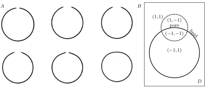
We represent an open vesicle using two labeling functions. We define a function
φ(x,t) by labeling the interior aqueous region, a diffuse interface containing the mem-brane, and outer aqueous region−1,0,and 1.Continuing, we define ¯φ(x,t) by labeling the part of the diffuse interface corresponding to water and the part corresponding to lipid by−1 and 1 respectively. φ(x,t) = 0 and ¯φ(x,t) = 1 impliesxis a lipid and otherwisexis a water. The role of the labeling functions is illustrated in figure 3.1 B. The use of multiple order parameters in the diffusive interface framework has en-joyed successful application in studying morphologically complex materials and mix-tures [12, 23, 28]. Our use of two labeling functions to describe the dynamics of an open vesicle in a fluid differs from these approaches in several respects. The labeling functions define an aqueous region interior and exterior to the vesicle, the bilayer, and the aqueous pore region. The dynamics of a lipidic pore is a non-equilibrium prob-lem with a well defined exchange of energy from stretching to pore enlargement, and viscosity limited outflow. Since our model consistently reproduces the experimentally recorded opening and closing of a lipid pore, we believe our particular treatment of the kinematic relationships is the appropriate way to model a rich set of hydrodynamic membrane morphological changes.
scales were proposed. To our knowledge, there are no three dimensional continuum simulations which describe open vesicles in solution.
The details of the diffusive interface energy are given in Section 2. The equations of motion are defined in Section 3. We used modified transport equations for φ(x,t) and ¯φ(x,t) that properly reflect the kinematics of the membrane and pore. These important details, as well as the derivation of the force, are discussed in Section 3. In Section 3.1, we use the scaling relationships of the energy to derive the nondimensional coefficients. Section 4 gives the simulation results visualizing the membrane shape, water motion, and dissipation of energy, as well as comparison with experimental results. Details of the discretization method are also found there.
Finally, we remark that biological membranes and vesicles are complicated mate-rials involving several components and multi-scale interactions. The problem we are considering here deals with a highly simplified membrane model system. Although vesicles can be quite complicated structures, for brevity we will refer to a fluid com-partment formed by the simple bilayer as a vesicle.
The challenge is to know how nature solves the problems of membrane construc-tion and vesicle dynamics. Since we do not know what resoluconstruc-tion is needed to describe the features of the bilayer, our approach is to use a rather simple model, and then as it fails to reproduce specific important experimental phenomena, to add additional structural features, e.g., inner and outer lipid leaflets, proteins, and see how the ad-ditions help explain the data.
2. Diffusive interface functional
In this section, we introduce functionals used to approximate the classical contin-uum lipid membrane energy. Define the cutoff functions
α(p) =1
2(tanh(ξp) + 1), α¯(p) = sech 2
(ξp), ξ >0.
The role of these cut-off functions will be explained below. Define the functionals
A= 3
2√2 Z
D α( ¯φ)
ǫ
2|∇φ| 2
+1
ǫF(φ)
dx, (2.1)
W= 3
4√2 Z
D α( ¯φ)ǫ
∆φ−ǫ12F′(φ) 2
dx, (2.2)
L=9 8 Z
D
ǫ
2|∇φ| 2
+1
ǫF(φ) ǫ
2|∇φ¯| 2
+1
ǫF( ¯φ)
dx. (2.3)
Here D is the three dimensional computational domain. The functionF(p) =1 4(p
2 − 1)2 is a double welled potential and ǫ is a small, positive parameter related to the thickness of the diffuse interface. The functionalW approximates the mean curvature squared energy of the membrane surface, L approximates the circumference of the pore, andAapproximates the membrane surface area. Define
˜
E=bW+jL+s(A−Ar)
2
2Ar
+wA. (2.4)
˜
Eapproximates the Helfrich energy of the vesicle. The first term in (2.4) is the bending energy of the vesicle. It is the energetic contribution coming from the splay of the lipid molecules [10]. The second term is the edge energy1
. When a pore is formed, lipid
1We distinguish between the terms line energy and edge energy. The former refers to the energy
molecules reorient so that the hydrophilic head groups shield the membrane interior from water. The edge energy is proportional to pore circumference. The third term is a Hookean relationship accounting for the mechanical energy stored in excess area. It can also be used in a penalty formulation to enforce the constraint A=Ar. Here,
Aris the area of the unstretched membrane. The membrane is inextensible when the mechanical moduluss is large. The last term is surface energy. The coefficients b,j
andware the bending modulus, edge tension, and surface tension respectively. In (2.1) and (2.2), the integrands are multiplied byα( ¯φ) so that only the compo-nent of the interface corresponding to membrane contributes to the total energy. In (2.3), the factors in the integrand approximate the area density of the two interfacial regions defined by φand ¯φ. The rim of the pore is located along the intersection of these regions. The product of the respective area densities in (2.3) yields a satisfactory approximation of the circumference of the pore.
To stabilize the method, we use the energy
E= ˜E+m1 2 P
2
+m2W ,¯ (2.5)
where
¯
W= 3
4√2 Z
D ǫ
∆ ¯φ−ǫ12F′( ¯φ) 2
dx, P=
Z
D
(∇φ·∇φ¯)2dx (2.6)
are auxiliary functionals. Here m1 is a penalty parameter for the constraint P= 0. This constraint leads to orthogonal interfaces. The prefactorm2is a small, stabilizing parameter. In the sequel,EφandEφ¯denote the Euler-Lagrange derivative ([7]) ofE with respect toφand ¯φ,respectively.
The following identities will be used to deriveb,j,s,andwfrom known, physical constants. Let D=R3 and for λ >0, define φλ and ¯φλ by a dilation of space and defineǫλ=λǫ.Making the change of variables yields
Aλ=λ 2
A, Lλ=λL, Wλ=W. (2.7)
Here, the subscript λ is used to denote the functionals’ dependence on φλ, φ¯λ, and ǫλ.
3. Equations of motion
To study the time course of the pore, we must evaluate the velocity of the mem-brane and aqueous solution. The velocity is determined by the equations of motion:
ut+u·∇u+∇p−η∆u=f, (3.1)
divu= 0, (3.2)
φt+α( ¯φ)u·∇φ=−γEφ, (3.3)
¯
φt+ ¯α(φ)u·∇φ¯=−¯γEφ¯, x∈D, t >0. (3.4)
Here, uis the velocity of a water molecule in the water region and the velocity of a lipid molecule in the membrane. pis the pressure. Equations 3.1 and 3.2 comprise the Navier-Stokes equations. The force exerted by the diffusive interface is given by
f=α( ¯φ)Eφ∇φ+ ¯α(φ)Eφ¯∇φ.¯ (3.5)
that the internal friction of the fluid, whether water, lipid, or at the water lipid in-terface, is Newtonian with a constant viscosityη.The viscosity of lipid membrane is typically greater than that of the solution. However, the membrane is very thin (a few nanometers) when compared to the overall geometry of the vesicle. Thus, the vis-cous dissipation in the membrane is much smaller than in the bulk aqueous medium. As the densities of water and lipid are comparable, we assume a constant density. Equations 3.3 and 3.4 are stabilized transport equations stemming from the condition that the labeling functions are carried by the fluid. The numbersγ and ¯γ are small, positive stabilizing constants.
Equations (3.1-3.5) are complemented by the initial conditions u(x,0) =u0(x), divu0= 0,φ(x,0) =φ0(x),and ¯φ(x,0) = ¯φ0(x).On the boundary, we assume a no-slip condition for the velocity and natural boundary conditions for the labeling functions:
u(x,t) = 0, φ(x,t) = ¯φ(x,t) = 1, ∂φ ∂n(x,t) =
∂φ¯
∂n(x,t) = 0, x∈∂D,t >0, (3.6)
where ∂
∂n is the outward normal derivative on∂D.
Cut-off functions are used to modulate the convective term in the transport equa-tions. In equation 3.3, the convective term is multiplied by the cut-off functionα( ¯φ).
As a result, φ is convected only where ¯φ takes positive values. In particular, the region of the diffusive interface inside the pore is not affected by the efflux of water. In equation 3.4, the label ¯φis convected where φ takes values close to zero, that is, along the rim of the pore.
Equation 3.5 is derived using the principle of virtual work. The derivation is a modification of techniques developed in [6]. The modification deals mainly with defining a suitable variation of the domain based on the kinematic conditions described in the previous paragraph.
A B
lipid
pore
(−1,1)
(1,1)
(−1,−1)
(1,−1)
[image:5.612.81.432.442.598.2]D
Fig. 3.1. (A) Cross sections of a vesicle with a hole as a function of time. (B) Illustration of
the pore defined by a pair of labeling functions(φ(x),φ¯(x)).The diffusive interface{φ≈0}is drawn by a solid line and the diffusive interface{φ¯≈0}is drawn by a dashed line.
The constantsb,s,j andware defined by
b= 106b0τ2
ρ0λ5
, j= 109j0τ2
ρ0λ4
, s= 1012s0τ2
ρ0λ3
, w= 1012w0τ2
ρ0λ3
. (3.7)
Here b0 pNnm is the experimentally measured bending modulus, s0 pNnm−1 the stretching modulus,j0 pN the edge tension,w0 pNnm−1 the surface tension, andρ0 gcm−3the density of the solution. A realistic bending modulus is 20 pNnm and real-istic surface tension is 1 pNnm−1.As an illustration, a giant vesicle in an experiment can typically be tens of microns in diameter and changes can occur over a time course seconds long. This scale yields a b on the order of 0.1 and w on the order of 107
.
The difference in magnitude of these constants suggests that bending, compared to surface tension, is irrelevant for the dynamics of large vesicles. To contrast, biological vesicles have diameters in the tens to hundreds of nanometers. Only in this regime and smaller are the constants bandwthen comparable.
Lethu,p,φ,φ¯ibe a smooth solution of equations (3.1-3.6). Form the dot product equation (3.1) withuand integrate overD.Multiply (3.3) byEφand (3.4) byEφ¯and integrate overD.Integrating by parts using (3.2) and (3.6) then gives the energy law
d dt
Z
D 1 2|u|
2
dx+E
+
Z
D
η|∇u|2+γ|Eφ| 2
+ ¯γ|Eφ¯|2dx= 0. (3.8)
The details of a related calculation may be found in [4, 5]. Using (2.7), make the change of variables ˆt=τ ts, ˆx=λx µm, and ˆǫ=λǫ µm. Matching the coefficients in (3.8) with the dimensional coefficients b0,s0,j0, and w0 then yields (3.7). Readily apparent from this calculation is η= 109
η0τ(ρ0λ2)−1, where η0 cP is the dynamic viscosity of the solution.
4. Simulation results
4.1. Discretization. To simulate the vesicle through equations (3.1-3.6), a spatial discretization by the finite difference method was developed. We simplified the problem to two dimensions by assuming a cylindrical geometry. Stretched vesicles with pores are axially symmetric, as can be seen in the experimental images of [11]. We assumed the vesicle was located in the rectangle (0,1)×(0,L). A fully implicit, backward Euler scheme was used in the time integration. For simplicity, the convective term was dropped from the Navier-Stokes equation. This assumption was justified by the fact the Reynolds number of flow in these biological systems is on the order of 10−2.
A Picard iteration between the Stokes system and the parabolic sub-systems was used to solve for the velocity-pressure pair and the diffusive interface transport equations simultaneously. The Stokes system was solved using the preconditioned conjugate gradient routine found in [9], Algorithm 22.7.3. A mixed Picard-Newton’s method was used to deal with the gradients of the discrete functional and the con-vective term. The linear systems were solved by SSOR preconditioned conjugate gra-dients. The stabilizing coefficientsǫγ andǫγ¯ were small when compared to (∆tk)−1
.
The condition number of the Jacobian resulting from the discretization of stabilized transport equations was consequently not large. The algorithm was implemented in
C.
0 4 8 12 16
0 1 2 3 s
log(kT)
A
0 4 8 12 16
0 1 2 3 s
log(kT)
[image:7.612.97.396.82.199.2]B
Fig. 4.1. Energy as a function of time. (A) In the rapid opening stage, mechanical energy
(hashed curve) is converted into kinetic energy (dashed curve) and edge energy (solid curve). Bend-ing energy (dotted curve) is relatively constant. The kinetic energy increases briefly in the rapid closing stage. (B) Total energy is nonincreasing.
geometry of the vesicle. For the time integration, a uniform time step ∆tk= 10−4 was used. The stability of the time integration, large fluid viscosity, stabilization parameters, and small step size ensured the monotonicity of energy. At each time the total energy was seen to be nonincreasing (figure 4.1 B). The radius of the pore was calculated by averaging ther-coordinate of the overlap of the two diffusive interfaces. In the numerical experiments, the constraint and stability constants wereγ= ¯γ= 10−2,
m1= 103,andm2= 0.1 respectively.
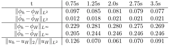
t 0.75s 1.25s 2.0s 2.75s 3.5s
kφh−φHkL2 0.097 0.085 0.081 0.079 0.077 kφ¯h−φ¯HkL2 0.012 0.018 0.021 0.021 0.021 kφh−φHkL∞ 0.229 0.281 0.280 0.275 0.269
kφ¯h−φ¯HkL∞ 0.205 0.244 0.246 0.246 0.246
kuh−uHk2/kuHkL2 0.126 0.070 0.061 0.070 0.091
Table 4.1.Mesh independence: Comparison of simulation on128×256and64×128grids.
Numerical tests were performed to check the sensitivity of the simulation with respect to the grid size and with respect to the auxiliary parameters. In the first test, the simulation variablesφh,φ¯h,and uh defined on a fine, 128 by 256 grid were compared against the simulation variables φH, φ¯H, and uH defined on a coarse, 64 by 128 grid. In both cases the computational domain was (0,1)×(0,2) and all other physical parameters and auxiliary parameters were the ones used in the experimental setup described in Section 4.2. In order to keep the diffusive interface thickness constant, ǫwas set to 6∆xon the fine grid and to 3∆xon the coarse grid. In table 4.1, we see that the fine and coarse grid solutions differ by roughly 10% in the L2
-norm throughout the range of the simulation. The labeling functions differ in the
L∞-norm by roughly 20%, implying that the position of the diffusive interface differs
by only a few grid points. In particular, the position of the vesicle and velocity are stable with respect to the grid size. To show that the dynamic is governed primarily by the diffusive interface energy, we also explored the dependence on the auxiliary constants. We compared the simulation whenγ= ¯γ= 10−2, m
1= 103, and m2= 0.1, the values used in the numerical experiments, against the simulation with the altered valuesγ= ¯γ= 2·10−2, m
[image:7.612.118.394.374.449.2]0 1 2 3 4
0 1 2 3 4 s
µm
A
r
r r rrr rr rr r r r r r rr r r
r r r rr r r r rr r rr
r r r r r r r r r r
r r rr r r rrr r r r rr r
r r r rrr r rr r r
r r r r r rr
r
r
0 1 2 3 4
0 1 2 3 4 s
µm
[image:8.612.75.414.75.201.2]B
Fig. 4.2. Experimental and simulated pore radius as a function of time. (A) Microscopy data
[1] for a vesicle of radius 20µm in solution with η0= 20cP. (B) The same vesicle simulated with
s0= 0.045, w0= 0, b0= 20, j0= 2.5, τ= 0.1, η0= 30,andλ= 40.Solid line: γ= ¯γ= 10−2, m1= 103,
andm2= 0.1.Dashed line: γ= ¯γ= 2·10−2, m1= 0.5·103,andm2= 0.2.
as a function of time for two sets of values forγ, ¯γ, m1, andm2 in figure 4.2 B. The solid line corresponds to the values used in the numerical experiment while the dashed line corresponds to the altered values. We see that the overall dynamic is not greatly effected by doubling and halving the auxiliary values.
The fluid was assumed initially at rest. The vesicle was initially a sphere with radius half of the domain. A pore was introduced by defining a sphere one twentieth the radius of the domain, centered at the pole of the vesicle. Our model does not spontaneously form a pore. The opening and closing of the pore involves the geometry of the lipid molecules at a length scale a few nanometers in diameter, much smaller than considered by classical continuum mechanical models. The exact mechanism governing the opening and closing of a pore is itself an interesting subject and is beyond the scope of this study. See, for example, [27].
4.2. A large vesicle with infoldings. In the experimental practice of creating and visually recording a pore, a large vesicle tens of microns in diameter is placed in solution. These vesicles are not taut, but have small undulations while maintaining an overall spherical shape. A mechanical tension is introduced by the photoactivation of fluorescently labeled lipids which in turn leads to an excess of area. The two dimensional modulus typically associated with this unfolding is s0= 0.045. Furthermore, a solution with viscosity several times that of water is used to slow and make the experiments easier.
In order to compare the diffusive interface model with the classical experimental result [1], we chose a solution viscosity 30 times that of distilled water. The spatial scale λ was chosen so the initially spherical vesicle had a radius of 20 µm and the surrounding cylindrical fluid region a radius of 40 µm and height 80 µm. We used the realistic values b0= 20 and j0= 2.5 for the bending modulus and edge tension respectively. For this experiment, unfolding is more consequential than surface tension and so we setw0= 0.
A B C
[image:9.612.74.443.108.356.2]D E F
Fig. 4.3. (A) Initially, mechanical tension widens the pore. (B) In the transition from stage
one to stage two, mechanical tension is relaxed. (C) In the the closing stages, edge tension closes the pore. For clarity, only one third of the arrows are plotted. (D) Initially the flow is concentrated in the pore but quickly develops around the pore. (E,F) In the closing stages, flow is more in plane with the pore.
a spatially constant multiple of the surface normal, is orders of magnitude larger than bending and edge tension. Thus, the increase in energy associated with a deviation from a spherical shape is much larger than the change in energy associated with the widening and closing of the pore. Many biological vesicles are much smaller than this, as we shall soon see, some as small as 50 nm. The effect of surface tension is more pronounced for smaller vesicles. Note that in this experiment, the diffusive interface represents the apparent location of the membrane. The undulations occurring at a much smaller length scale are not resolved.
4.3. Comparison and discussion. The simulation captures the experimen-tally well known, three stage form of the pore radius as function of time. Preceding the first stage, a mechanical tension is imposed by assuming the vesicle has an excess area of four percent ([11]). A small pore is introduced. The presence of the pore permits the vesicle to lose area. As seen in figure 4.3 A, a rapid widening, stage one, is induced by diffusive interface forces pointing away from the pore. In figure 4.3 D, fluid leaks from the interior of the vesicle. In figures 4.1 A and 4.2 B, one sees that the maximum radius is reached and most of the energy dissipated in one tenth of the life-time of the pore.
0.00 0.01 0.03 0.04 0.06
0.0 1.0 2.0 3.0 4.0 µs
A
0.0 6.0 12.0 18.0 24.0
0.0 1.0 2.0 3.0 4.0 µs
nm
[image:10.612.75.397.74.199.2]B
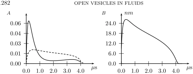
Fig. 4.4. Simulation results for an osmotically swollen vesicle of radius 50 nm in solution
η0= 1,withs0= 60, w0= 1, b0= 20, j0= 2.5, τ= 10−8,andλ= 0.1.(A) Percent leak out of vesicle
volume (solid line) and sphericity (dashed line). Sphericity is defined asA/As−1, whereAs is the
area of the spherical zone with the identical volume and pore radius as the vesicle. (B) Pore radius as a function of time.
the fluid. The rate of contraction is quite small when compared to stage one. The pore dynamic concludes with the third, rapid closing stage. As the pore becomes smaller, the curvature increases which in turn increases the radial force due to edge tension, accelerating the pore closure. The water in the interior of the vesicle, no longer affected by Laplace pressure, is almost completely static. The pore seals due to diffusive effects of the interface. This occurs when the radius of the pore is comparable to the diffusive interface thickness.
4.4. A small osmotically stretched vesicle. The creation of a pore by osmotic swelling is a process with considerable interest to biologists. Hemolysis, the leaking out of the contents out of a red blood cell, has been studied and observed by clinicians for centuries. Encouraged by the agreement of the simulation with exper-imental data for large vesicles, we proceed to simulate a small, osmotically swollen vesicle.
Due to dimensional scaling, small vesicles can withstand the large pressure associ-ated with osmotic gradients by increasing their area slightly. The stretching modulus
s0= 60 associated with the excess area per lipid is much larger than the one due to unfolding ([13]). The stretching tension plus the surface tensionw0= 1 for submicron vesicles results in a significant Laplace pressure.
We simulated a vesicle with radius 50 nm in a solution of distilled water. In order to resolve the time course, we chose a time scale tenths of microseconds long by setting τ= 10−8
by the low Reynolds outflow though the pore.
5. Sharp interface limit
Under suitable modeling assumptions, the energy of the open vesicleEenjoys the sharp interface limit
E0= Z
Mt
(bH2
+w)α0dS+s
(|Mt|α0−Ar) 2
2Ar
+j|Mt∩M¯t|+m2 Z
¯ Mt
H2
dS. (5.1)
Here Mt and ¯Mt are smooth, closed, orthogonal surfaces evolving with t and where Mt∩M¯t represents the rim of the pore. When ξ is large, the function α0(x,t) is a positive, step wise function taking values close to 1 exterior to ¯Mtand values close to 0 interior to ¯Mt.By|Mt|α0we denote that approximate area ofM,namely the surface integral ofα0 overM. By|Mt∩M¯t|we denote the length of the intersection. HereH is the mean curvature ofMtor ¯Mtand as beforem2is a small, stabilizing parameter. Thus the diffusive interface model converges to the classical Helfrich energy of a lipid bilayer with a hole plus auxiliary terms for the surfaces used to label the position of the hole.
The modeling assumptions are
φ(x,t) =q(d(x,t)/ǫ) +ǫg1(x,t) +ǫ2g2(x,t) +...,
¯
φ(x,t) = ¯q( ¯d(x,t)/ǫ) +ǫ¯g1(x,t) +ǫ2 ¯
g2(x,t) +...,
whered(x,t) and ¯d(x,t) are the signed distance function to smooth, closed, transverse surfaces Mt and ¯Mt in D respectively. The surfacesMt and ¯Mtare the boundaries of the sets of points where φand ¯φ are positive respectively, in the limit ǫ= 0. The functions qand ¯qdescribe the limiting profile of the labeling functions and g1,g2,g¯1, and ¯g2 are smooth functions independent ofǫ.We also assume thatE is bounded by a constant independently ofǫand the other modeling parameters. This assumption is reasonable since the energy is known (by the dissipation relation (3.8)) to be bounded by the energy of the initial vesicle.
In [5, 6, 28], a related problem was analyzed for a single diffusive interface ap-proximation of the Willmore–mean curvature squared–energy with surface area and volume constraints. Using the assumptions stated above, Theorems 2.1 and 2.2 of [5] imply that thatq(r) = ¯q(r) = tanh(r/√2) andg1≡¯g1≡0.Summarizing the argument, the energyEis expanded in powers ofǫ.Collecting the lowest order terms, the energy remains bounded providedqand ¯qare solutions to the ordinary differential equation
q′′−q(q2
−1) = 0.The boundary conditions (3.6) then imply thatqand ¯qare profiles given by the hyperbolic tangent function. The remaining terms in the expansion of
E involves the square norm ofg1 and ¯g1.These terms are bounded independently of
ǫprovided g1 and ¯g1 are identically zero. By making only slight modifications to ac-count for the termαappearing in the integrand ofW andA,we can apply Theorem 4.1 of [5] to recover the sharp interface limit for the surface integrals appearing in (5.1).
It remains to show that the diffusive interface approximationLconverges to the length of the rim of the pore|Mt∩M¯t|.The constraint functionalPwas introduced in [28] to ensure that the diffusive interfaces are effectively orthogonal. We use expansion and the boundedness ofP to conclude thatMtand ¯Mtare orthogonal. Note that the gradient of the distance functions are a multiple of the unit normalsnand ¯nofMtand
¯
of the curveMt∩M¯t, the first term in the expansion ofP in ǫis bounded below by
cǫ−4Z Mt∩M¯t
(n·n¯)2
dl
for some constant c independent of ǫ. Since this quantity is bounded independently ofǫ,we infer thatMtand ¯Mtare orthogonal. Using Lemma 2.2 of [5], the remaining terms in the expansion of P vanish with ǫ. Thus, the boundedness of P and the asymptotic assumptions imply that limǫ→0P= 0.
The orthogonality of sharp interface limits is now sufficient to imply that the approximation L actually converges to the length of the rim of the pore. This is achieved by first assuming that Mt∩M¯t is piecewise linear and passing to the limit ǫ= 0.The general case follows by approximation and noting that, with the asymptotic assumptions,Lis uniformly continuous with respect to Lipschitz deformations of the curve Mt∩M¯t. Consider the rectangular cylinder Q={(x1,x2,x3) : 0< x3< l,−√ǫ <
x1,x2<√ǫ}.Assume, without loss of generality, thatMt∩M¯t∩Qlies in thex3-axis andnand ¯nare parallel with the coordinate directions. This assumption is possible since the interfaces are orthogonal. Asǫ approaches 0, the signed distance functions
dand ¯dare uniformly approximated by the coordinate functionsx1andx2.Using the identities F(p) = (p2
−1)2 = (p′)2
/2 and limǫ→0 R√ǫ
−√ǫ 1 ǫq′(s/ǫ)
2
ds=2√32, we evaluate the limit
lim ǫ→0 Z
Q
ǫ
2|∇φ| 2
+1
ǫF(φ) ǫ
2|∇φ¯| 2
+1
ǫF( ¯φ)
dx=8 9l=
8
9|Mt∩M¯t∩Q|.
To calculate the entire length, coverMt∩M¯tby a union of such cylinders, noting that the integrand vanishes exponentially on the exterior of the cover, and the contribution from the overlap vanishes in the limitǫ= 0.This show that limǫ→0L=|Mt∩M¯t|.This concludes the demonstration of the sharp interface limit (5.1).
6. Conclusion
The diffusive interface model captures the dynamic shape of an open vesicle where the membrane and water is impelled by surface and line forces. The numerical method is stable, encompasses a wide range of length and time scales through scaling parame-ters, and is capable of producing realistic time courses of vesicles and their flow fields below the experimentally observable limits. The simulation results for large vesicles are in good quantitive agreement with classical experiments. The model converts large amounts of energy stored in mechanical stretching into fluid motion, edge en-ergy, and heat. The simulations indicate that the overall shape of the vesicle remains sphere-like throughout the time course.
The model was unable to produce a pore spontaneously. An initial, small pore was assumed and sealing is an artifact of the diffusive interface representation. Future work will study functionals for which spontaneous pore formation is an energy minimizing path.
REFERENCES
[1] F. Brochard-Wyart, P.G. de Gennes, and O. Sandre,Transient pores in stretched vesicles: role
of leakout, Physica A, 278, 32–51, 2000.
[2] G. Caginalp and X. Chen,Convergence of the phase field model to its sharp interface limits,
Eur. J. Appl. Math., 9, 417–445, 1998.
[3] Q. Du, C. Liu, and X. Wang, A phase field approach in the numerical study of the elastic
bending energy for vesicle membranes, J. Comput. Phys., 198, 450–468, 2004.
[4] Q. Du, M. Li, and C. Liu, Analysis of a phase field Navier-Stokes vesicle-fluid interaction
model, DCDS B, 8, 539–556, 2007.
[5] Q. Du, C. Liu, R.J. Ryham, and X. Wang,A phase field formulation of the Willmore problem,
Nonlin., 18, 1249–1267, 2005.
[6] Q. Du, C. Liu, R.J. Ryham, and X. Wang,Energetic variational approaches in modeling vesicle
and fluid interactions, Physica D, 238, 9-10, 923–930, 2009.
[7] L.C. Evans,Partial Differential Equations, AMS Graduate Studies in Mathematics, 1991.
[8] L.C. Evans and H.M. Soner, Phase transitions and generalized motion by mean curvature,
Commun. Pure Appl. Math., XLV, 1097–1123, 1992.
[9] R. Glowinski, P.G. Ciarlet, and J.L. Lions,Handbook of Numerical Analysis: Numerical
Meth-ods for Fluids, 9, 3, 2003.
[10] W. Helfrich,Elastic properties of lipid bilayers-theory and possible experiments, Zeitschrift f¨ur
Naturforschung C, 28, 693–703, 1973.
[11] E. Karatekin, O. Sandre, H. Guitouni, N. Borghi, P.-H. Puech, and F. Brochard-Wyart,
Cas-cades of transient pores in giant vesicles: line tension and transport, Biophys. J., 84,
1734–1749, 2003.
[12] J. Kim and J. Lowengrub,Phase field modeling and simulation of three-phase flows, Inter. Free
Bound., 7, 4, 435–466, 2005.
[13] P.I. Kuzmin, S.A. Akimov, Y.A. Chizmadzhev, J. Zimmerberg, and F.S. Cohen,Line tension
and interaction energies of membrane rafts calculated from lipid splay and tilt, Biophys.
J., 88, 1120–1133, 2005.
[14] Y. Levin and M.A. Idiart,Pore dynamics of osmotically stressed vesicle, Physica A, 331, 571–
578, 2004.
[15] J.S. Lowengrub, J.-J. Xu, and A. Voigt,Surface phase separation and flow in a simple model
of multicomponent, Fluid Dynamics and Materials Processing, 3, 1, 1–19, 2007.
[16] L. Modica,The gradient theory of phase transitions and the minimal interface criterion, Arch.
Rat. Mech. Anal., 98, 2, 123–142, 1987.
[17] R. Moser, A higher order asymptotic problem related to phase transitions, SIAM J. Math.
Anal., 37(3), 712–736, 2005.
[18] J.D. Moroz and P. Nelson,Dynamically stabilized pores in bilayer membranes, Biophys. J., 72,
2211–2216, 1997.
[19] P.-H. Puech and F. Brochard-Wyart, Membrane tensiometer for heavy giant vesicles, Eur.
Phys. J. E, 15, 127–132, 2004.
[20] T. Portet and R. Dimova, A new method for measuring edge tension and stability of lipid
bilayers: effect of membrane composition, Biophys. J., 99, 3264–3273, 2010.
[21] M. R¨oger and R. Sch¨atzle,On a modified conjecture of DeGiorgi, Mathematische Zeitschrift,
254(4), 675–714, 2006.
[22] J.S. Sohn, Y.-H. Tseng, S. Li, A. Voigt, and J. Lowengrub, Dynamics of multicomponent
vesicles in a viscous fluid, J. Comput. Phys., 229, 119–144, 2010.
[23] H. Sun, J.J. Brannick, C. Liu, and T. Qian,Diffuse interface method for multiple phase
mate-rials: An Energetic Variational Approach, preprint, 2011.
[24] S.H. Veerapaneni, Y.-N. Young, P.M. Vlahovska, and J. B lawzdziewicz, Dynamics of a
com-pound vesicle in shear flow, Phys. Rev. Lett., 106, 158103, 2011.
[25] P.M. Vlahovska, Y.-N. Young, G. Danker, and C. Misbah,Dynamics of a non-spherical
micro-capsule with incompressible interface in shear flow, J. Fluid Mech. 678, 221–247, 2011.
[26] J.D. Van der Waals,Thermodynamic theory of capillarity assuming continuous change of
den-sity, Natuurk. Verb. Kon. Akad. Amsterdam 1, 1–56, 1892.
[27] J. Wohlert, W.K. den Otter, O. Edholm, and W.J. Briels,Free energy of a trans-membrane pore
calculated from atomistic molecular dynamics simulations, J. Chem. Phys., 124, 154905,
2006.
[28] X. Wang and Q. Du,Modeling and simulations of multi-component lipid membranes and open
![Fig. 4.2.[1] for a vesicle of radiussand0 =0 m Experimental and simulated pore radius as a function of time](https://thumb-us.123doks.com/thumbv2/123dok_us/8111184.236418/8.612.75.414.75.201/fig-vesicle-radiussand-experimental-simulated-pore-radius-function.webp)