Design of a Repetitive Controller as a Feed-forward
Disturbance Observer
M. Tang, A. Formentini, S. Odhano, P. Zanchetta
The University of Nottingham, University ParkNottingham, UK
Email: [email protected]
Abstract—From the structure point of view, a repetitive controller (RC) is considerably similar to a disturbance observer. By adding a correction term to the traditional RC and considering the disturbances as states, the repetitive controller can be designed in the same way as a disturbance observer. This paper presents therefore a new simple way of tuning a repetitive controller. Simulations show that, when compared with the traditional RC, the proposed RC configuration can achieve greater stability margin. As opposed to the traditional plug-in RC, the new RC structure studied in this paper is also shown to be robust against variations in the inner loop delays if it is used in a cascaded configuration. The immunity to plant parameter variations is another added benefit of the proposed controller.
Keywords—control design, discrete-time system, disturbance observer, reduced-order observer, repetitive control, stability analysis, state estimation
I. INTRODUCTION
The repetitive controller (RC) is an effective solution for rejecting periodic disturbances in closed loop control systems for several reasons [1-17]. Among those, one of the key pros of the repetitive control is the fact that the controller can be designed by only knowing the frequency of the disturbance. However, every coin has two sides; due to lack of information about the plant, the design of the controller can be challenging in terms of stability. For example, some main causes of instability can be the parameter variations of controlled plant, which modify the gain and phase of the whole system; or variation of the plant delays, which consequently causes unwanted phase shift between reference and response (output). Therefore, for the sake of robust performance, careful considerations should be given to the design of repetitive controllers. Some of the most commonly used tuning methods for repetitive control are based on the H-infinity control [1, 2], Lyapunov function [3-5], Routh-Hurwitz stability criterion [6], Nyquist stability criterion [7], small gain theorem [7, 8], pole placement [9] and other optimization methods in robust control [10, 11].
Besides, depending on the type of uncertainties contained in the plant, it may be also necessary to enhance the robustness of the repetitive controller with some other adjustments in the control design. Some examples of the adjustments are given as following:
(1) For disturbances with varying period, one solution is to use variable sampling frequency: a strategy for calculating
the sampling frequency is proposed in [12], whereas an RC compensator proposed in [10] can maintain the stability while the sampling frequency is varying. Alternatively, for drive applications, since the period of disturbances is a function of rotor position, an angle-based RC is proposed in [13].
(2) For non-periodic disturbances, a repetitive signal filter, which removes non-periodic components, is presented in [14]; an equivalent input disturbance estimator which provides better attenuation to aperiodic disturbances is presented in [15].
(3) For parametric uncertainties, it is common to use an observer in conjunction with the repetitive controller [2, 4, 5, 14, 16] to estimate uncertain states. In such way, taking advantage of the learning ability of the repetitive controller, the system is able to operate stably under parametric uncertainties.
Moreover, the observer can be a state observer (SO), an extended state observer (ESO) or a disturbance observer (DO), depending on the availability of the states from the measurements.
Authors in [16] have shown that, instead of SO which only estimates system states, the ESO which also estimates disturbance as an additional state can work better with the repetitive controller for rejecting external disturbances.
It is also worth noting that, the RC and DO are similar since they both can help rejecting external disturbances by learning the disturbances. Authors in [14] have shown that the RC proposed in their paper converges faster than a DO.
However, none of the works presented so far have considered that, in case of a plug-in repetitive controller, the structure becomes almost the same as a disturbance observer without correction term. By adding the correction term to the traditional RC, and considering the disturbance as an additional state like in the ESO, this paper proposes a novel methodology for designing the repetitive controller as a reduced-order disturbance observer. Therefore, the tuning of the RC is decoupled from the tuning of the plant controller.
In the following paper, Section II presents the equations and design procedure of the proposed RC with the correction term. Section III presents the comparison simulation results for an example plant with the proposed RC and the traditional RC, along with stability analysis. Section IV finally provides some conclusions.
II. DESIGN OFRCASDO
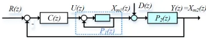
[image:2.595.61.273.101.141.2]Let us consider a typical two cascaded loops control system as shown in the block diagram in Fig. 1.
Fig. 1. The block diagram of a typical two cascade loops control system
Where, P1(z) represents the inner loop as a whole, P2(z)
represents the plant for the outer loop,C(z)is the controller for the outer loop, R(z), U(z), D(z), and Y(z) are the outer loop reference, inner loop reference, disturbance, and output respectively. Xm1(z) and Xm2(z)are the measurable subspaces
used as the inner and outer loop feedbacks respectively. The design procedure for RC can be broken down into the following three subsections.
A. Equation Derivation for DO
Before we can design the RC like a DO, it is worth now to write the equation for the DO.
First, the state space equations for the dynamic system from inputU(z)to outputY(z)in Fig. 1 can be written as (1).
1 11 12 1 1
2 21 22 2
1 2
( 1) ( )
( )
( 1) ( ) 0
0 ( )
( ) ( ) 0 1
( )
m m
m m
m m
X k a a X k b
U k
X k a a X k
D k A X k Y k X k (1)
a11, a12, a21, a22 and b1 are matrices of appropriate
dimensions according to the dimensions ofXm1andXm2.Ais a
coefficient shows how the disturbance D(k)would affect X
m2-(k+1). If the disturbance D(z) is periodic, and can be modelled as the sum of sine wave of frequency fdand all its
multiple, its resulting dynamical model is
33
( 1) ( ) ( ) ( )
d d
d d
X k a X k
D k c X k
(2)
where
33
0 1 0 0 0 0 0 0 1 0 0 0 0 0 0 0 0 0
0 0 0 0 1 0 0 0 0 0 0 1 1 0 0 0 0 0 1 0 0 0 0 0
d a c (3)
The disturbance Xd is a vector of N elements, where the
relationN=fs/fd must hold.fsis the sampling frequency of the
control system.
Second, by combining system (1) and (2), (4) shows a state space equation where the disturbanceXd(k)can be seen as an
additional state of the system.
1 11 12 1 1
2 21 22 2
33 1 2
( 1) 0 ( )
( 1) ( ) 0 ( )
( 1) 0 0 ( ) 0
( ) ( ) 0 1 0 ( ) ( )
m m
m d m
d d
m m d
X k a a X k b
X k a a A c X k U k
X k a X k
X k
Y k X k
X k (4)
Rewriting the second and third lines of (4) we obtain
2 21 1 22 2
33
( ) ( 1) ( ) ( )
( 1) ( )
d d m m m
d d
A c X k X k a X k a X k
X k a X k
(5)
Third, the estimated disturbance equation can then be derived from (5) as a reduced order observer.
33
2 21 1 22 2
ˆ ( 1) ( ) ˆ ( )
( 1) ( ) ( )
d d d
m m m
X k a L A c X k
L X k L a X k L a X k
(6)
whereLis a vector ofNgains,L1,L2…LN-1,LN.
B. Modification of RC to Resemble DO
According to (6), the block diagram for DO is drawn in Fig. 2 (a). Comparing to the traditional repetitive controller [17] as shown in Fig. 2 (b), it can be seen from the orange part that a feedback of the previous output, which yields a correction term in the input is included in DO, while this correction term is missing in the traditional RC.
(a) DO according to (6)
[image:2.595.313.559.155.250.2] [image:2.595.317.546.564.694.2]Apart from the correction term, the structures of the green parts in both diagrams in Fig.2 are actually similar to each other. Therefore, the block diagram of the proposed RC that combines the traditional RC and the correction term of DO is developed as shown in Fig.3.
Fig. 3. The block diagram of the proposed RC with correction term
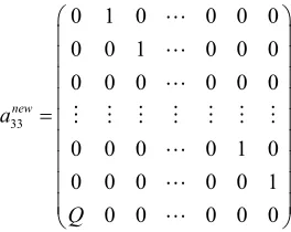
In order to include the forgetting factorQof the standard repetitive controller as shown in Fig.2(b) in the matrixa33as
shown in Fig. 2(a), matrixa33has been modified from (3) to
(7).
33
0 1 0 0 0 0 0 0 1 0 0 0 0 0 0 0 0 0
0 0 0 0 1 0 0 0 0 0 0 1 0 0 0 0 0
new a
Q
(7)
The stability filter in Fig. 2 (b) is chosen to be a simple time advance filterzM, i.e. the equivalent delay introduced by
the inner loopP1(z)and the feedback path. To model it in the
[image:3.595.318.552.151.233.2]state space representation, the Qf block has been added in
Fig.3, which is a one-by-N vector of zeros with only the Mth
value equals to 1. Effectively, this time advance filter chooses one value from the estimated disturbance vectorܺௗ.
C. Tuning RC as a DO
Following the design in Fig.3, it can be noticed that the proposed RC becomes the same structure of a disturbance observer, and thus shall share the same equation (6) with the DO. Therefore, the poles of the proposed RC can be determined by the eigenvalues of the matrix(a33-LAcd)in (6)
or matrix (a33new-LAcd) to include the forgetting factor Q.
Hence, the gain vector L for the correction term can be designed by choosing the roots of (8). As can be seen from (8), the choice of L also depends on the choice of Q. Further discussions will be given in part III.
200 19933 1
198
2 199 200
det
0 new
d
I a L A c A L
A L A L A L Q
(8)
III. SIMULATION ANDSTABILITYANALYSIS
The simulation model is built using Matlab/Simulink. For comparison, both the new control scheme model of Fig. 3 and the one of the traditional plug-in RC [17] shown in Fig. 4 have been built. To be distinguishable by the quantities defined for the proposed RC, G and F are defined as the gain and the forgetting factor of the traditional RC respectively. URC2(z)
andYRC2(z)are the input and output of RC.
Fig. 4. The block diagram of the plug-in traditional RC
A simple system (9) is considered to perform a comparison analysis between the proposed RC and its traditional version. The inner loop is assumed to be a delay of two sampling periods. The main frequencies of the periodic disturbances are 50 Hz and 300 Hz. The sampling frequency is 10 kHz, N is 200 (i.e. 10k/50).Mis designed to be 3 since there is a delay of 3Tsfrom the output of RCYRC(z)being applied to the inner
loop till the reading of the corresponding outcomes are measured and transmitted back to RC.
2
1( ) , ( ) 0.1282 (2 0.9999) ( ) sin(100 ) 0.5sin(600 )
P z z P z z
D z t t
(9)
It can then be calculated from (9) that:
21 0.1282, 22 0.9999, 0.1282
a a A (10)
The bandwidth of the outer loop is chosen to be 100Hz and the outer loop controllerC1(z)is designed as a PI controller.
1( ) (0.3658 0.3597) / ( 1)
C z z z (11)
Moreover, (8) is simplified by choosingL1=L2=…= L199=0.
Therefore, the root location of λ only depends on the selection
of gain L200 and forgetting factor Q. For locating the root
inside the unity circle, the choice needs to meet the following criteria:
200 200
| | 1
1 1
Q AL
Q Q
L
A A
[image:3.595.84.216.293.398.2]Despite the stability margin, the selection of gainL200and
forgetting factor Qalso need to consider the performance as analyzed below.
A. Choosing L200and Q for the Best Performance
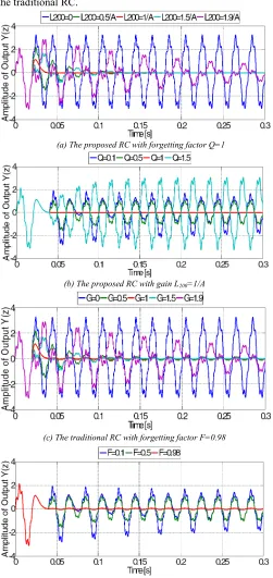
The outputsY(z)with different gains and forgetting factors are compared in Fig.5 using the model of the proposed RC and the traditional RC.
(a) The proposed RC with forgetting factor Q=1
(b) The proposed RC with gain L200=1/A
(c) The traditional RC with forgetting factor F=0.98
[image:4.595.39.290.168.699.2](d) The traditional RC with gain G=1 Fig. 5. The response of the output Y(z) to disturbance D(z)
Fig. 5 (a) shows the influence of gainL200on the outputY(z)
using the proposed RC model of Fig. 3, while Fig. 5 (b) shows the influence of the forgetting factorQ. It can be seen thatL200
mainly affect the convergence time and Q mainly affect the steady state value. The best performance is obtained when L200=1/AandQ=1so that the poles of the proposed RC are all
located at the origin of z-plane (λ=Q-AL200=0).
Fig. 5 (c) and (d) show the influence of gain G and forgetting factorFon the outputY(z)using the traditional RC model of Fig. 4. It can be seen that the gain and forgetting factor affect the response almost in the same way in both models. However, the system is unstable if F ≥1 in the traditional RC model since all the poles will be located on the edge or outside the unity circle of z-plane (see later in (14)). Therefore, by reducingF, the stability can be maintained, but the performance is sacrificed.
B. Gain and Delay Margin at the Best Performance
The best performance setting of L200 and Q has been
confirmed above. It is now necessary to verify the resultant gain and delay margins with such setting.
The open loop transfer functionsGOP1(z)andGOP2(z)from
inputR(z)to outputY(z)are derived according to Fig. 3 as (13) and Fig. 4 as (14) in order to analyze the stability margins:
1
1 1 2
22 1 1 2 21 1 1
200 1
200 ( )
( ) ( ) ( )
1 (1 ) ( ) ( ) ( ) ( ) ( ) ( ) ( ) ( )
1 OP
RC RC
N M
RC RC RC N
G z
C z P z P z
a z G z P z P z a zG z P z
L z
G z Y z U z
AL Q z
(13)
1 1 2 2
2 1 1
2 1 2 2
2 2 2
( ) ( ) ( ) 1 ( )
1 ( ) ( ) ( ) ( ) ( ) ( ) ( )
1
RC OP
RC
N M
RC RC RC N
C z P z P z G
G z
G z P z P z z P z Gz
G z Y z U z
Fz
(14)
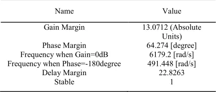
The gain and delay margins are computed using Matlab functions from the control toolbox. The proposed RC achieves the results in Table 1 by settingL200=1/AandQ=1. The results
for the traditional RC when setting G=1 andF=0.98are not shown since the poles are close the unity circle, and the software fails to compute the stability margins.
The results in Table 1 prove three main advantages of the proposed RC:
The system can still maintain stable behavior even when the open loop gain increases by 13 times or the open loop delays increase for 22 more sampling periods! In the example, the inner loop P2(z)is assumed to be a
delay of 2Ts, which is true if a deadbeat control is
[image:4.595.319.563.375.530.2]when the deadbeat control is at its physical limit. Since, even at physical limit, the delay of the deadbeat control loop is unlikely to be more than 24Ts, the results prove
the stability of the system against the delay variation in the inner loop.
Meanwhile, taking benefit from the large gain and phase margin, the system is also reasonably robust against parameter variations in the plant.
In addition, designing the repetitive controller as a disturbance observer permits to decouple the tuning of the RC from the tuning of the plant controller due to the principle of separation of estimation and control. For verifying the stability region and comparing with the traditional RC, the outputsY(z)using the proposed RC and the traditional RC with increased system gain and delay are shown in Fig.6. The gain and delay of the system is modified through the transfer function of the inner loop plant P2(z). The gains
and forgetting factors for both the proposed and traditional RC are chosen to be the combinations that give the best performance in Fig.5. Therefore, L200=1/A, Q=1, G=1,
F=0.98.
(a) The proposed RC with the gain and delay of system both increase for 3.65dB and 16Ts
[image:5.595.325.542.338.431.2](b) The proposed RC and traditional RC with only the delay of system increase for Ts
Fig. 6. The response of the output Y(z) with increased gain and delay in the system
The results in Fig.6 show that with the gain and delay increased for 3.65dB (=1.5 Absolute Units) and 16Ts in the
plant, the effectiveness of the proposed RC consequently degrades, but the system is still stable. However, the system with traditional RC fails to maintain the stability even when the inner loop delays for only one more sampling period. Therefore, the traditional RC used in the paper is more
sensitive to delay variations in the open loop system than the proposed RC.
IV. CONCLUSION
A new way of designing repetitive controller has been presented in this paper. The traditional repetitive controller is modified to resemble a reduced order observer so that the gain and forgetting factor of the repetitive controller can be tuned following the same procedure of tuning an observer. Stability analysis shows that the proposed repetitive controller can achieve large stability margins without sacrificing the performance, and the proposed controller is stable against variations of delays and parameters in the plant.
The performance of this new RC configuration is compared with the traditional RC structure, and it is found that the proposed controller is able to cope with delay and parameter deviations, which would push the traditional controller to the limits of stability.
The authors are working on implementing the proposed control on a test rig to better highlight its advantage over existing schemes.
REFERENCES
[1] M. Wu, L. Zhou, and J. She, "Design of Observer-Based H-infinity Robust Repetitive-Control System," IEEE Transactions on Automatic Control, vol. 56, pp. 1452-1457, 2011.
[2] A. Noshadi, S. Juan, L. Wee Sit, S. Peng, and A. Kalam, "Repetitive disturbance observer-based control for an active magnetic bearing system," in Control Conference (AUCC), 2015 5th Australian, 2015, pp. 55-60.
[3] E. Kurniawan, C. Zhenwei, and M. Zhihong, "Digital design of adaptive repetitive control of linear systems with time-varying periodic disturbances," IET Control Theory & Applications, vol. 8, pp. 1995-2003, 2014.
[4] W. E. Dixon, E. Zergeroglu, D. M. Dawson, and B. T. Costic, "Repetitive learning control: a Lyapunov-based approach," IEEE Transactions on Systems, Man, and Cybernetics, Part B (Cybernetics), vol. 32, pp. 538-545, 2002.
[5] X. Jian-Xin and X. Jing, "Observer based learning control for a class of nonlinear systems with time-varying parametric uncertainties," IEEE Transactions on Automatic Control, vol. 49, pp. 275-281, 2004. [6] C. Weijie, X. Fangchun, W. Min, and S. Jinhua, "Design of a repetitive
control system based on the compensation of nonlinearities," in Control Conference (CCC), 2013 32nd Chinese, 2013, pp. 182-186.
[7] J. Chao, P. Zanchetta, F. Carastro, and J. Clare, "Repetitive Control for High-Performance Resonant Pulsed Power Supply in Radio Frequency
TABLE I
RESULTS OFSTABILITYMARGINANALYSIS
Name Value
Gain Margin 13.0712 (Absolute Units) Phase Margin 64.274 [degree] Frequency when Gain=0dB 6179.2 [rad/s] Frequency when Phase=-180degree 491.448 [rad/s]
Delay Margin 22.8263
Applications," IEEE Transactions on Industry Applications, vol. 50, pp. 2660-2670, 2014.
[8] X. H. Wu, S. K. Panda, and J. X. Xu, "Design of a Plug-In Repetitive Control Scheme for Eliminating Supply-Side Current Harmonics of Three-Phase PWM Boost Rectifiers Under Generalized Supply Voltage Conditions," IEEE Transactions on Power Electronics, vol. 25, pp. 1800-1810, 2010.
[9] M. Yamada, Z. Riadh, and Y. Funahashi, "Design of discrete-time repetitive control system for pole placement and application," IEEE/ASME Transactions on Mechatronics, vol. 4, pp. 110-118, 1999. [10] E. Kurniawan, C. Zhenwei, and M. Zhihong, "Design of Robust
Repetitive Control With Time-Varying Sampling Periods," IEEE Transactions on Industrial Electronics, vol. 61, pp. 2834-2841, 2014. [11] E. Kurniawan, Z. Cao, and Z. Man, "Design of decentralized repetitive
control of linear MIMO system," in Industrial Electronics and Applications (ICIEA), 2013 8th IEEE Conference on, 2013, pp. 427-432.
[12] P. Zanchetta, M. Degano, J. Liu, and P. Mattavelli, "Iterative Learning Control With Variable Sampling Frequency for Current Control of Grid-Connected Converters in Aircraft Power Systems," IEEE Transactions on Industry Applications, vol. 49, pp. 1548-1555, 2013. [13] Y. Yuan, F. Auger, L. Loron, S. Moisy, and M. Hubert, "Torque ripple
reduction in Permanent Magnet Synchronous Machines using
angle-based iterative learning control," in IECON 2012 - 38th Annual Conference on IEEE Industrial Electronics Society, 2012, pp. 2518-2523.
[14] C. Xu and M. Tomizuka, "New Repetitive Control With Improved Steady-State Performance and Accelerated Transient," IEEE Transactions on Control Systems Technology, vol. 22, pp. 664-675, 2014.
[15] M. Wu, B. Xu, W. Cao, and J. She, "Aperiodic Disturbance Rejection in Repetitive-Control Systems," IEEE Transactions on Control Systems Technology, vol. 22, pp. 1044-1051, 2014.
[16] A. H. M. Sayem, C. Zhenwei, M. Zhihong, and F. Chaohong, "Performance comparison of SO and ESO based RC," in Systems, Process & Control (ICSPC), 2013 IEEE Conference on, 2013, pp. 121-124.