Design and Development of Classification Model
for Recyclability Status of Trash Using SVM
Adwait Arayakandy1, Ankit Gupta2, Rashmi Thakur3
1, 2, 3
Computer Department, Thakur College of Engineering & Technology, Mumbai, India.
Abstract: SVM are a relatively new supervised classification technique for the cartographic community of land cover. They have their roots in statistical learning. SVMs are inherently essentially binary classifiers. Our classification problem involves
receiving images of a single object and classifying it into a recycling material type. The input to our pipeline is images in which a single object is present on a clean white background.
Keywords: SVM; hyperplane; machine learning;
I. INTRODUCTION
Recycling is important for a sustainable society. The current recycling process requires recycling facilities to sort garbage by hand and uses arrangement of huge channels to separate out more distinct objects. Consumers can also be confused about how to determine the correct way to dispose of a wide variety of materials used in packaging.
This input to this project are images of a single piece of recycling or garbage, process them and classify it into six classes consisting of glass, paper, metal, plastic, cardboard, and trash. In order to mimic a stream of materials at a recycling plant or a consumer taking an image of a material to identify it, our classification problem involves receiving images of a single object and classifying it into a
recycling material domain. The input to our pipelines is images in which a single object is present on a clean white background. We then use an SVM to classify the image into six categories of garbage classes. By using machine learning algorithm, we can predict the category of garbage that an object belongs to base on just an image. This will have beneficial economic effects and also positive environmental effects.
II. RELATEDWORK
III.SUPPORTVECTORMACHINE
SVM is a supervised learning model which is used for classification and regression analysis. For image classification it uses linear separable algorithm. Linear separable algorithm is used to determine a pair set of sets is linearly separable and finding a separating hyperplane if they are arising in several different areas. If they arise in same area it means they are same object.
Fig.1: Block diagram of SVM
The first analysis used an SVM to classify waste into recycling categories. The SVM was chosen because it is considered one of the best initial classification algorithms and is not so complicated compared to a CNN. The SVM classifies the elements by defining a hyphen separation plane for multidimensional data. The hyperplane that the algorithm tries to find is the hyperplane, which offers the largest minimum distance to the training examples. More specifically, an SVM’s optimization objective is
min (γ, w, b)1/2 ||w||2
s.t y (i) (w T x (i) + b) ≥ 1, i = 1, ..., m
where w, b are parameters of our hypothesis function, y (i) represents the label for a specific example, x (i) is the i th example out
of m, and γ is the minimum geometric margin of all training examples. For a multiclass SVM, a common method is a one versus all
classification where the class is chosen based on which class model classifies the test datum with greatest margin.
The features used for the SVM were SIFT features. At a high level, the SIFT algorithm finds features like bubbles in an image and describes them in 128 numbers.
In particular, the SIFT algorithm passes a Gaussian filter difference that varies the values of σ as an approximation to the Gaussian
Laplacian. The values σ are used to identify larger and larger areas of an image. Next, the images are searched for local extremes through scale and space. A pixel in an image is compared to neighbours of different scales. If the pixel is a local endpoint, it is a potential key point. This also means that the key point is better represented on this specific scale. Once the potential key points have been found, they must be refined through the extension and threshold of the Taylor series. Then, each key point is given an orientation to achieve invariance in the rotation of the image. The key point is rotated in 360 directions, represented as a histogram in 36 containers (10 degrees per container), depending on the size of the gradient for certain rotations. The key point is selected as the rotation with the largest number of values in a container. Once the key point is found, a 16x16 environment is captured around the key point. Then it is subdivided into 16 blocks of size 4x4. For each sub-block, an 8-bin orientation histogram is created. So, there is a total of 128 container values available. The characteristics of SIFT are powerful because they are independent of scale, noise and lighting, which makes them ideal for reuse. Most recycled objects do not look very different, but they differ in size and colour.
Then a bag of functions was attached. The SIFT descriptors for the training images were grouped according to the k-mean algorithm, where k was the number of training examples. Then, for each new test example, the properties of SIFT are extracted and a histogram of values based on the original grouping is used as the data point for the data set. This significantly reduces the SVM training time required as an image is reduced to a histogram.
A. One Versus Rest Approach
The 1-versus-rest (1VR) approach constructs k separate binary classifiers for classification for k-class. The m-th binary classifier is trained using the data of the m-th class as positive examples and the remaining k-1 classes as negative examples. During the test, the class label is determined by the binary classifier that returns the maximum output value. A major problem with the approach to recovery is the unbalanced training set. Suppose all classes have the same training size. The proportion of positive and negative examples in each classifier is 1 k - 1. In this case, the symmetry of the original problem is lost.
B. One Versus One Approach
Another classical approach for multi-class classification is the one-versus-one(1V1) or pairwise decomposition. It evaluates all classifiers of possible pairs and therefore induces k (k-1) / 2 individual binary classifiers. Applying each classifier to a test example would give the victorious class a voice. A test example is marked for the class with the most votes. The size of the classifiers created by the one-to-one approach is much larger than the approximation to the rest. However, the QP size in each classifier is less so that training can be done quickly. Also, compared to the focus on recovery, the one-to-one method is more symmetrical. Platt et al. [28] improved the one-to-one approach and proposed a method called SVM (DAGSVM), which forms a tree structure to facilitate the testing phase. Therefore, only k-1 individual scores are required to determine the name of a test example.
IV.PURPOSEDWORK
An SVM was used for the first analysis to classify waste into recycling categories. The SVM was chosen because it is considered one of the best initial classification algorithms and is not so complicated compared to a CNN.The SVM classifies the elements by defining a hyperplane separator for multidimensional data. The hyperplane that the algorithm tries to find is the hyperplane, which offers the greatest distance to the training examples.
We are going to use software like MATLAB and programming languages like Python and R and machine learning libraries like Tensor Flow to create the Model.
Fig.4: Flowchart of SVM
We will use Mozilla image compressor for compressing the size of training images and testing images so that size of Model is compressed.
The proposed model will take image of a single piece of garbage and first determine whether it’s recyclable or non-recyclable and if it’s recyclable then classify it into six classes (glass, paper, metal, plastic, cardboard, and trash) with accuracy of more than 73%. We are going to use machine learning algorithm such as multiclass SVM (Support Vector Machine) as dataset have only images. In order to achieve more accuracy, we will focus on different image classification technique which help our algorithm to produce more accurate results.
V. RESULTANDDISCUSSION
Fig.5: Training Data set
For training the model, we have collected around 500 to 600 images of each categories of garbage. This entire collection of images is the data set for the model. Out of these images 80% of images are used for training the model and the remaining are use for testing the model.
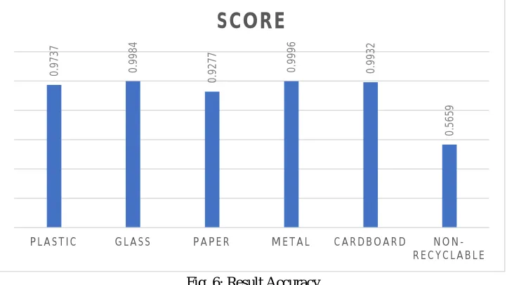
[image:4.612.190.420.76.233.2]We train the model for all the categories of garbage and achieved an accuracy of 79.7%. then we tested the model for each category and the result for each is given below:
Fig. 6: Result Accuracy
We have trained our model multiple times with different number of images each time and following are the accuracy achieved: Number of training images Accuracy (in %)
100 81.1
200 85.3
300 83.5
400+ 86.4
Table 1: Accuracy
VI.CONCLUSIONANDFUTURESCOPE
The sorting of garbage into different categories of recycling is possible through machine learning and computer vision algorithms. One major issue is the wide variety of possible data (i.e. each object can be assigned to one of the waste or recycling categories). Therefore, to create a more accurate system, there must be a large and growing data source.
It can classify a single image of waste into six categories (Plastic, Metal, Paper, Glass, Cardboard and Trash). In future it would be able to classify garbage from a multi
object image. It can also would be able to classify from video data.
0 .9 7 3 7 0 .9 9 8 4 0 .9 2 7 7 0 .9 9 9 6 0 .9 9 3 2 0 .5 6 5 9
[image:4.612.126.487.318.521.2]REFERENCES
[1] Mindy Yang and Gary Thung,”Classification for Recyclability status.”,in Stanford University,pp.2016.
[2] J. Donovan,“Auto-trash sorts garbage automatically at the techcrunch disrupt hackathon.”,in Tech-Crunch Disrupt Hackathon,2016.
[3] G.Mittal,K.B. Yagnik,M. Garg,and N.C. Krishnan, “Spotgarbage: Smartphone app to detect garbage using deep learning,”in Proceedings of the 2016 ACM International Joint Conference on Pervasive and Ubiquitous Computing , ser. UbiComp ’16. New York, NY, USA: ACM, 2016, pp. 940–945.
[4] S. Zhang and E. Forssberg, “Intelligent liberation and classification of electronic scrap,” Powder technology, vol. 105, no. 1, pp. 295–301, 1999.
[5] C. Liu, L. Sharan, E. H. Adelson, and R. Rosenholtz, “Exploring features in a ayesian framework for material recognition,” in Computer Vision and Pattern Recognition (CVPR), 2010 IEEE Conference on. IEEE, 2010, pp. 239–246.