Global Solutions to DSGE Models as a Perturbation of a Deterministic Path

Munich Personal RePEc Archive

Global Solutions to DSGE Models as a

Perturbation of a Deterministic Path

Ajevskis, Viktors

Bank of Latvia, Riga Technical University

8 April 2014

Online at

https://mpra.ub.uni-muenchen.de/55145/

Global Solutions to DSGE Models as a

Perturbation of a Deterministic Path

Viktors Ajevskis

Bank of Latvia and Riga Technical University

[email protected]

April 8, 2014

Abstract

This study presents an approach based on a perturbation technique to construct global solutions to dynamic stochastic general equilibrium models (DSGE). The main idea is to expand a solution in a series of pow-ers of a small parameter scaling the uncertainty in the economy around a solution to the deterministic model, i.e. the model where the volatility of the shocks vanishes. If a deterministic path is global in state variables, then so are the constructed solutions to the stochastic model, whereas these solutions are local in the scaling parameter. Under the assump-tion that a deterministic path is already known the higher order terms in the expansion are obtained recursively by solving linear rational expecta-tions models with time-varying parameters. The present work proposes a method rested on backward recursion for solving this type of models.

Key words: DSGE, perturbation method, rational expectations models with time-varying parameters, asset pricing model

1

INTRODUCTION

Perturbation methods are the most widely-used approach to solve nonlinear DSGE models owing to their ability to deal with medium and large-size models for reasonable computational time. Perturbations applied in macroeconomics are used to expand the exact solution around a deterministic steady state in powers of state variables and a parameter scaling the uncertainty in the economy. The solutions based on the Taylor series expansion are intrinsically local, i.e. they are accurate in some neighborhood (presumably small) of the deterministic steady state. Out of the neighborhood, for example, in the case of sufficiently

∗_{I thank the WGEM ECB participants, Rudolfs Bems and Anton Nakov for useful}

large shocks (or under the initial conditions that are far away from the steady state) the approximated solution can imply explosive dynamics, even if the original system is still stable for the same shocks (or initial conditions) (Kim, Kim, Schaumburg, and Sims(2008);Den Haan, and De Wind(2012)).

This study presents an approach based on a perturbation technique to con-struct global solutions to DSGE models. The proposed solutions are represented as a series in powers of a small parameter σ scaling the covariance matrix of the shocks. The zero order approximation corresponds to the solution to the deterministic model, because all shocks vanish as σ = 0. Global solutions to deterministic models can be obtained reasonably fast by effective numerical methods1_{even for large size models (Hollinger(2008)). For this reason the next}

stages of the method are carried out under the assumption that the solution to the deterministic model under given initial conditions is known.

The higher-order systems depend only on quantities of lower orders, therefore can be solved recursively. The homogeneous part of these systems is the same for all orders and depends on the deterministic solution. Consequently, each system can be represented as a rational expectation model with time-varying parameters. In the case of rational expectations models with constant parame-ters the stable block of equations can be isolated and solved forward. This is not possible for models with time-varying parameters. The present work proposes a method for solving this type of models. The method starts with finding a finite-horizon solution by using backward recursion. Next we prove that under certain conditions as the horizon tends to infinity the finite-horizon solutions approach to a limit solution that is bounded for all positive time.

If the parameterσis small enough, then the solutions obtained are close to the deterministic solution. At the same time, whenever the deterministic solu-tion is global in state variables so is the approximate solusolu-tion to the stochastic problem. For this reason, we shall call this approach semi-global, whereas the perturbation methods based on series expansion around the steady state will be referred to as local. In contrast to the solutions obtained by the local perturba-tion methods, the soluperturba-tions provided by the semi-global method inherit “global” properties, such as monotonicity and convexity, from the exact solution and thus cannot explode by construction.

We apply the method to the asset pricing model ofBurnside (1998). Since the model has a closed-form solution we can check the accuracy of an approx-imate solution against the exact one. We compare the accuracy of the second order solution of the semi-global method with the local Taylor series expansion of order two (Schmitt-Groh´e, and Uribe(2004)). The semi-global approach in-dicates superior performance in accuracy and inherits global properties from the exact solution.

This paper contributes to a growing literature on using the perturbation technique for solving DSGE models. The perturbation methodology in

eco-1_{The algorithms incorporated in the widely-used software such as Dynare (and less available}

nomics has been advanced by Judd and co-authors as inJudd(1998);Gaspar, and Judd (1997);Judd, and Guu(1997). Jin, and Judd (2002) give a theoret-ical basis for using perturbation methods in DSGE modeling; namely, applying the implicit function theorem, they prove that the perturbed rational expecta-tions solution continuously depends on a parameter and therefore tends to the deterministic solution as the parameter tends to zero.

Almost all of the literature is concerned with the approximations around the steady state as inCollard, and Juillard (2001); Schmitt-Groh´e, and Uribe

(2004); Kim, Kim, Schaumburg, and Sims(2008);Gomme, and Klein (2011).

Lombardo (2010) uses series expansion in powers of σ to find approximations to the exact solution recursively. Boroviˇcka, and Hansen (2013) employ Lom-bardo’s approach to construct shock-exposure and shock-price elasticities, which are asset-pricing counterparts to impulse response functions. This approach has some similarity with that employed in the current paper. However, both papers apply the expansion only around the deterministic steady state, therefore the solution obtained remains local. Lombardo’s approach can be treated as a spe-cial case of the method proposed in this study, namely a deterministic solution around which the expansion is used is only the steady state.

Judd (1998, Chapter 13) outlines how to apply perturbations around the known entire solution, which is not necessarily the steady state. He considers the simple continuous and discrete-time stochastic growth models in the dynamic programming framework. This paper develops a rigorous approach to construct solutions to DSGE models in general form by using the perturbation method around a global deterministic path.

The rest of the paper is organized as follows. The next section presents the model. Section3 provides a detailed exposition of series expansions for DSGE models. In Section 4 we transform the model into a convenient form to deal with. Section5presents the method for solving rational expectations models for time-varying parameters. The proposed method is applied to an asset pricing model in Section6, where it also compared with the local perturbation method in terms of accuracy. Conclusions are presented in Section7.

2

The Model

DSGE models usually have the form

Etf(yt+1, yt, xt+1, xt, zt+1, zt) = 0, (2.1)

zt+1= Λzt+σεt+1, εt+1∼N(0,Ω), (2.2)

whereEtdenotes the conditional expectations operator, xt is annx×1 vector containing thet-period endogenous state variables; yt is an ny×1 vector con-taining thet-period endogenous variables that are not state variables; zt is an

assumed to be sufficiently smooth. The scalarσ(σ >0) is a scaling parameter for the disturbance termsεt. We assume that all mixed moments ofεtare finite. All eigenvalues of the matrix Λ have modulus less than one.

The solution to (2.1) and (2.2) is of the form:

yt=h(xt, zt), (2.3) wherehmapsRnx_×Rnz _intoRny_{. Another way of stating the problem to solve}

is to say: for a given initial condition (x0, z0) find the initial condition y0 for

the vectory such that the solution (xt, yt) to (2.1)–(2.2) will be bounded for all

t >0.

3

Series Expansion

In this section we shall follow the perturbation methodology (see, for example,

Holmes(2013)) to derive an approximate solution to the model (2.1)–(2.2). For smallσ, we assume that the solution has a particular form of expansions

yt=

∞

X

n=0

σn_y(n)_{(xt, zt) (3.1)}

xt=

∞

X

n=0

σn_x(n)

t , (3.2)

where y(i)_{(xt, zt) andx}(i)

t , i = 0,1,2, . . . ,are the i-order of approximation to

the solution (2.3) and the variable xt, respectively. The exogenous processzt

can also easily be represented in the form of expansion inσ

zt=z_t(0)+σz_t(1). (3.3) Indeed, plugging (3.3) into (2.2) gives

zt+1=z_t(0)+1+σz (1)

t+1 = Λ(z (0)

t +σz

(1)

t ) +σεt+1.

Collecting the terms of like powers ofσand equating them to zero, we get

zt(0)+1= Λz (0)

t , (3.4)

zt(1)+1= Λz (1)

t +εt+1. (3.5)

Since the expansion (3.3) must be valid for all σat the initial time t= 0, the initial conditions are

z₀(0)=z0 and z0(1)= 0. (3.6)

Note that the arguments of the functions y(i) _{are expansions in powers of σ.}

yt=

∞

X

i=0

σi_y(i)





∞

X

j=0

σj_x(j)

t , z

(0)

t +σz

(1)

t



. (3.7)

Expandingytfor smallσand collecting the terms of like powers, we have

yt=

∞

X

n=0

σny∗(n)(x(0)t , x

(1)

t , ..., x

(n)

t , z

(0)

t , z

(1)

t ), (3.8)

where

y∗(0)(x(0)_t , z_t(0)) =y(0)(x(0)_t , z_t(0)), y∗(1)(x(0)t , x

(1)

t , z

(0)

t , z

(1)

t ) =y(1)(x

(0)

t , z

(0)

t ) +y

(0) 1,0;tx

(1)

t +y

(0) 0,1;tz

(1)

t ,

and

y∗(n)_(x(0)

t , x

(1)

t , ..., x

(n)

t , z

(0)

t , z

(1)

t ) =y

(n)_(x(0)

t , z

(0)

t ) +y

(0) 1,0;tx

(n)

t +pn,t, (3.9)

where the mapping pn,t = pn(x(0)t , x

(1)

t , . . . , x

(n−1)

t , z

(0)

t , z

(1)

t ) has arguments

with superscript less thannand is defined as

pn,t = n X l=0 1 l!

n−l

X

j=0

n−j−l

X

k=1

1

k!y

(j)

k,l;t





X

i1+i2+···+ik=n−j−l

n−j−l i1;i2;...;ik

x(i1)

t , x

(i2)

t , ..., x

(ik)

t ,

zt(1)

l 



Herey_k,l(j)_;tdenotes the mixed partial derivative ofy(j)_{of orderkandl with}

re-spect toxtandzt, respectively, at the point (x(0)t , z

(0)

t ), and

z(1)t

l

= (zt(1), . . . , z

(1)

t )

(l times). In other words,y(_k,lj)_;tis a (k+l)-multilinear mapping (see, for exam-ple,Abraham, Marsden, and Ratiu(2001, p. 55)) depending on (x(0)t , z

(0)

t ) (and

hence ont). Substituting (3.9) into (3.8), we can rewrite (3.8) as

yt=

∞

X

n=0

σnhy(n)(x(0)t , z

(0)

t ) +y

(0) 1,0;tx

(n)

t +pn,t

i

. (3.10)

Then substituting (3.2), (3.3) and (3.10) into (2.1), collecting the terms of like powers ofσand setting their coefficients to zero, we have

Coefficient of σ0

fy(0)(x(0)t+1, z (0)

t+1), y(0)(x (0)

t , z

(0)

t ), x

(0)

t+1, x (0)

t , z

(0)

t+1, z (0)

t

= 0, (3.11)

The requirement that (3.2) and (3.3) must hold for all arbitrary smallσimplies that the initial conditions for (3.11) are

z(0)₀ =z0 and x(0)0 =x0. (3.12)

(2.2), where all shocks vanish. The deterministic model (3.4) and (3.11) with the initial conditions (3.12) can be solved globally by a number of effective algorithms, for example the extended path method (Fair, and Taylor(1983)) or a Newton-like method (for example,Juillard(1996)). As this study is primarily concerned with stochastic models, in what follows we suppose that the solution (x(0)t , y(0)(x

(0)

t , z

(0)

t )) for t >0 to the deterministic model is already known.

Coefficient of σn_{, n >0}

Etnf1,t+1·yt(+1n) +f2,t+1·yt(n)+

h

f1,t+1·y(0)1,0;t+1+f3,t+1

i

x(tn+1)

+hf2,t+1·y1(0),0;t+f4,t+1

i

x(tn)+η

(n)

t+1

o

= 0, (3.13)

where y(tn) = y(n)(x

(0)

t , z

(0)

t ). The requirement that (3.2) must hold for all

arbitrary smallσimplies that the initial condition for (3.13) is

x(0n)= 0. (3.14)

The matrices

fi,t+1 =fi

y(0)(x(0)t+1, z (0)

t+1), y(0)(x (0)

t , z

(0)

t ), x

(0)

t+1, x (0)

t , z

(0)

t+1, z (0)

t

, i= 1, . . . ,6,

are the Jacobian matrices of the mappingf with respect to yt+1,yt, xt+1,xt,

zt+1, andzt, respectively, at the point

y(0)_(x(0)

t+1, z (0)

t+1), y(0)(x (0)

t , z

(0)

t ), x

(0)

t+1, x (0)

t , z

(0)

t+1, z (0)

t

.

The mappingEtη(tn)is of the form: Etη_t(n₊₁) =Etη(n)_x(0)

t+1, x (0)

t , . . . , x

(n−1)

t+1 , x (n−1)

t , z

(0)

t+1, z (0)

t , z

(1)

t+1, z (1)

t

,

whereη(n)_{is some mapping for which the set of arguments includes only}

quan-tities of order less thann. The vector z(1)_t+1 enters the expectations Etη_t(₊₁n) in the form of the mixed moments of ordernor less. The subscriptt+ 1 infi,t+1

andηt(n+1) reflects their dependence ont+ 1 throughx (0)

t+1andz (0)

t+1.

The expectationEtη_t(+1n) is bounded if all mixed moments ofz (1)

t+1are bounded

up to ordernand the vectors

y_t(0)+1, y (0)

t , x

(0)

t+1, x (0)

t , . . . , y

(n−1)

t+1 , y (n−1)

t , x

(n−1)

t+1 , x (n−1)

t , z

(0)

t+1, z (0)

t , z

(1)

t+1, z (1)

t

are bounded for allt≥0.

4

Transformation of the Model

Define the deterministic steady state as vectors (¯y,x,¯ 0) such that

f(¯y,y,¯ x,¯ x,¯ 0,0) = 0. (4.1)

We can represent fi,t+1 in (3.13) as fi,t+1 = fi+ ˆfi,t+1, i = 1, . . . ,6, where

fi=fi(¯y,y,¯ x,¯ x,¯ 0,0) are the Jacobian matrices of the mapping f with respect toyt+1,yt,xt+1, xt,zt+1, andzt, respectively, at the steady state, and

ˆ

fi,t+1=fi,t+1(y(0)t+1, y (0)

t , x

(0)

t+1, x (0)

t , z

(0)

t+1, z (0)

t )−fi(¯y,y,¯ x,¯ x,¯ 0,0). (4.2)

Note also that ˆfi,t+1→0 ast→ ∞, because a deterministic solution must tend

to the deterministic steady state asttends to infinity. Consequently,fi,t+1 can

be thought of as a perturbation offi.

To shorten notation, further on we omit the superscript (n) when no confu-sion can arise. Therefore Equations (3.13) can be written in the vector form

Φt+1Et

xt+1

yt+1

= Λt+1

xt yt

+Etηt+1, (4.3)

where Φt =

h

f3+ ˆf3,t, f1+ ˆf1,t

i

and Λt =

h

f4+ ˆf4,t, f2+ ˆf2,t

i

. We assume that the matrices Φt are invertible for all t≥0. This assumption holds if, for

example, the Jacobian [f3, f1]−1 at the steady state is invertible2and the terms

ˆ

f1,t and ˆf3,t are small enough for all t≥0. Pre-multiplying (4.3) by Φ−t+11 , we

get

Et

xt+1

yt+1

=L

xt yt

+Mt+1

xt yt

+ Φ−_t+11Etηt+1, (4.4)

whereL= [f3, f1]−1[f4, f2] and

Mt+1=

h

f3+ ˆf3,t+1, f1+ ˆf1,t+1

i−1h

f4+ ˆf4,t+1, f2+ ˆf2,t+1

i

−[f3, f1]−1[f4, f2].

Notice that limt→∞Mt = 0. As in the case of rational expectations models

with constant parameters it is convenient to transform (4.4) using the spectral property ofL. Namely, the matrixL is transformed into a block-diagonal one using the block-diagonal Schur factorization3

L=ZP Z−1, (4.5)

where

P =

A 0 0 B

; (4.6)

2_{This assumption is made for ease of exposition. If [f3, f1] is a singular matrix, then}

further on we must use a generalized Schur decomposition for which derivations remain valid, but become more complicated.

whereAandB are quasi upper-triangular matrices with eigenvalues larger and smaller than one (in modulus), respectively; andZis an invertible matrix4_{. We}

also impose the conventional Blanchard-Kan condition (Blanchard, and Kahn

(1980)) on the dimension of the unstable subspace, i.e., dim(B) =ny. After introducing the auxiliary variables

[st, ut]′ =Z−1[xt, yt]′ (4.7) and pre-multiplying (4.4) byZ−1_{, we have}

Etst+1=Ast+Q11,t+1st+Q12,t+1ut+ Ψ1t+1Etηt+1, (4.8)

Etut+1=But+Q21,t+1st+Q22,t+1ut+ Ψ2t+1Etηt+1, (4.9)

where [Ψ1,t+1,Ψ2,t+1] =ZΦ−t+11 and

Q11,t+1 Q12,t+1

Q21,t+1 Q22,t+1

=ZMt+1Z−1. (4.10)

System (4.8)-(4.9) is a linear rational expectations model with time-varying parameters, thus we cannot apply the approaches used in the case of models with constant parameters (Blanchard, and Kahn (1980); Anderson and Moor

(1985);Sims(2001);Uhlig(1999), etc.). In Subsection5.2we devevop a method for solving this type of models.

5

Solving the Rational Expectations Model with

Time-Varying Parameters

5.1

Notation

This subsection introduces some notation that will be necessary further on. By

|·|denote the Euclidean norm in Rn_{. The induced norm for a real matrixD is}

defined by

kDk= sup

|s|=1

|Ds|.

The matrixZ in (4.5) can be chosen in such a way that

kAk< α+γ <1 andkB−1k< β+γ <1, (5.1) whereαand β are the largest eigenvalues (in modulus) of the matrices Aand

B−1, respectively, andγ is arbitrarily small. This follows from the same argu-ments as in Hartmann (1982, §IV 9), where it is done for the Jordan matrix decomposition. Note also thatkBk−1<1 for sufficiently small γ. Let

Bt=B+Q22,t

4_{A simple generalized Schur factorization is also possible to employ here, but at the cost}

andAt=A+Q11,t.(5.2)By definition, put

a= sup

t=0,1,...

kAtk, b= sup

t=0,1,...

B−_t1

, (5.3)

c= sup

t=0,1,...

kQ12,tk, d= sup t=0,1,...

kQ21,tk. (5.4)

Here and in what follows we assume that all the matrices Bt, t = 0,1, . . . ,

are invertible. The numbers a, b, c and d depend on the initial conditions (x(0)₀ , z(0)₀ ). From the definitions of At, A, Bt, B, Q12,t and Q21,t and the

conditionlimt→∞(x(0)t , z

(0)

t ) = (¯x,0), it follows that

lim

t→∞c(x

(0)

t , z

(0)

t ) = 0, _tlim_→∞d(x

(0)

t , z

(0)

t ) = 0, (5.5)

lim

t→∞a(x

(0)

t , z

(0)

t ) =kAk<1, lim t→∞b(x

(0)

t , z

(0)

t ) =

B−1

<1.

This means thatcanddcan be arbitrary small and

a <1 and b <1 (5.6) by choosing (x(0)₀ , z₀(0)) close enough to the steady state.

5.2

Solving the transformed system

(

4.8

)

–

(

4.9

)

Taking into account notation (5.1), we can rewrite (4.8)–(4.9) in the form

Etst+1=At+1st+Q12,t+1ut+ Ψ1,t+1Etηt+1, (5.7)

Etut+1=Bt+1ut+Q21,t+1st+ Ψ2,t+1Etηt+1. (5.8)

In this subsection we construct a bounded solution to (5.7)–(5.8) fort≥0 with an arbitrary initial condition s0 ∈ Rnx and find under which conditions this

solution exists. For this purpose, we first start with solving a finite-horizon model with a fixed terminal condition using backward recursion. Then, we prove the convergence of the obtained finite-horizon solutions to a bounded infinite-horizon one as the terminal timeT tends to infinity.

Fix a horizon T > 0. Using the invertibility of BT=1 and solving

Equa-tion (5.8) backward, we can obtainuT as a linear function ofsT, the terminal conditionETuT+1 and the “exogenous” term Ψ2,T+1ETηT+1

uT =−B_T−+11 Q21,T+1sT −B_T−+11 Ψ2,T+1ETηT+1+B_T−+11 ETuT+1.

Proceeding further with backward recursion, we shall obtain finite-horizon so-lutions for eacht= 0,1,2, . . . , T.For doing this we need to define the following recurrent sequence of matrices:

KT ,T−i−1=LT−1+1,T−i(Q21,T−i+KT ,T−iAT−i), i= 0,1, . . . , T, (5.9)

where

with the terminal conditionKT ,T+1= 0. In (5.9) and (5.10) the first subscriptT

defines the time horizon, while the second subscript defines all times between 0 andT+ 1. LetuT ,T−i,i= 0,1, . . . , T,denote the (T−i)-time solution obtained

by backward recursion that starts at the timeT.

Proposition 5.1. Suppose that the sequence of matrices (5.9)and (5.10)exists; then the solution to (5.7)–(5.8) has the following representation:

uT ,T−i=−KT ,T−isT−i+gT ,i+ i+1

Y

k=1

L−_{T ,T}1_−i+k

!

ET−i(uT+1), (5.11)

wherei= 0,1, . . . , T;and

gT ,i=−

i+1

X

j=1

j

Y

k=1

L−_{T ,T}1_−i+k(Ψ2,T−i+j+KT ,T−i+jΨ1,T−i+j)ET−iηT−i+j. (5.12)

For the proof see Appendix A. The sequence of matrices (5.9) exists if all matricesLT ,T−i, i = 0,1, . . . , T, are invertible. For this we need, in addition,

some boundedness condition on the matricesB_T−₋1_iKT ,T−i+1Q12,T−i.

Proposition 5.2. If fora,b,canddfrom (5.3)–(5.4)the inequality

cd < 1

4

₁

b −a

2

=

_1−ab

2b

2

(5.13)

holds, then

B_T−₋1_i

· kKT ,T−i+1k · kQ12,T−ik<1, i= 0,1,2, . . . T. (5.14)

For the proof see AppendixA.

Proposition 5.3. If inequality (5.14) holds, then the matrices LT ,T−i, i =

0,1,2. . . . , T, are invertible.

Proof. From (5.10) and the invertibility ofBT−i it follows that LT ,T−i=BT−i I+BT−−1iKT ,T−iQ12,T−i

. (5.15)

The matricesLT ,T−iare invertible if and only if the matrices I+B_T−−1iKT ,T−iQ12,T−i

are invertible. From the norm property and (5.14) we have

B_T−₋1_iKT ,T−i+1Q12,T−i

≤

B−_T−1_i

· kKT ,T−i+1k · kQ12,T−ik<1.

Now the invertibility of I+B_T−−1iKT ,T−iQ12,T−i

follows fromGolub, and Van Loan (1996, Lemma 2.3.3)

Fori=T from (5.11) we have

uT ,0=−KT ,0s0+gT ,T +

T+1

Y

k=1

L−_{T ,k}1

!

This is a finite-horizon solution to the rational expectations model with time-varying coefficients (5.7)–(5.8) and with a given initial condition s0. What is

left is to show that the solutionuT ,0 of the form (5.16) converges to some limit

asT → ∞.

Proposition 5.4. If inequality (5.13)holds, then the limit

lim

T→∞KT ,j=K∞,j forj= 0,1,2, . . .

exists in the matrix space defined in Subsection5.1.

For the proof see AppendixA.

Proposition 5.5. If inequality (5.14)holds, then

lim

T→∞

T+1

Y

k=1

L−_{T ,k}1 = 0 (5.17)

and

lim

T→∞gT ,T =g∞, (5.18)

whereg∞ is some vector in Rny.

Proof. From (5.10) and Proposition5.4 it follows that

lim

T→∞LT ,k=Bk+K∞,kQ12,k=L∞,k.

Then the limit in (5.17) can be represented as

lim

T→∞

T+1

Y

k=1

L−_{T ,k}1 = lim

T→∞

T+1

Y

k=1

L−_∞1_,k. (5.19)

SinceK∞,k is bounded (it follows from formula (A.7) in AppendixA) and

lim

k→∞Q12,k= 0, and klim→∞B −1

k =B

−1_,

we havelimk→∞L−_∞1_,k=B−1. Therefore, ifδ >0 is arbitrary small, there is an

N=Nδ ∈N_{such that}

kL−_∞1_,kk ≤β+δ=ρ <1, (5.20)

fork > N, where β is the largest eigenvalue (in modulus) of the matrix B−1_.

From this, the norm property and (5.19) we obtain

lim

T→∞

T+1

Y

k=1

L−_{T ,k}1

≤ lim

T→∞

T+1

Y

k=1

L

−1

∞,k

≤ lim

T→∞C1ρ

T−K_{= 0,}

By (5.20) the products in (5.12) decay exponentially with the factor ρ as

j → ∞. From this and the boundedness of the terms KT ,k, Ψ2,k, Ψ1,k and E0ηk,T ∈Nandk= 1,2, . . . , T+ 1, it follows that the series

gT ,T =−

T+1

X

j=1

j

Y

k=1

L−_{T ,k}1(Ψ2,j+KT ,jΨ1,j)E0ηj.

converges to someg∞ asT → ∞.

From Proposition 5.4 and Proposition 5.5 it may be concluded that as T

tends to infinity Equation (5.16) takes the form:

u0=−K∞,0s0+g∞. (5.21)

Formula (5.21) gives us the unique bounded solution to the transformed rational expectation model with time-varying parameters (5.7)–(5.8). Note also that the proofs of Propositions5.2–5.5are based on inequality (5.13) that is a spectral gap condition for the unstable and stable parts of the system (5.7)–(5.8), and in a sense substitutes for the Blanchard-Kahn condition for rational expectations models with time-varying parameters. It follows from (5.3)–(5.6) that inequality (5.13) always holds if initial conditions (x(0)_t , z(0)_t ) is close enough to the steady state. Nonetheless, the condition (5.13) is not local by itself.

5.3

Restoring the original variables

x

and

y

Recall that we deal with the n-order problem (3.13)–(3.14), and now we put the superscript (n) back in notation. To find the bounded solution in terms of the original variablesx(tn)andy

(n)

t we need to obtain the initial valuesu

(n) 0 and

s(0n)that correspond to that of the problem (4.4), i.e. x (n)

0 = 0. From (4.7) and

(5.21) we have

"

s(0n)

−K∞(n,)0s (n) 0 +g

(n)

∞

#

=Z−1

₀

y0(n)

,

whereZ−1_{is a matrix that is involved in the block-diagonal Schur factorization}

(4.5) and has the following block-decomposition:

Z−1=

Z11 _Z12

Z21 _Z22

.

Hence

s(0n)=Z12y (n)

0 , (5.22)

−K∞(n,)0s (n)

0 +g(∞n)=Z22y

(n)

0 . (5.23)

Substituting (5.22) into (5.23) and assuming that the matrixZ22_+K(n)

∞,0Z12

is invertible, we get

y0(n)= (Z22+K (n)

The left-hand side of (5.24) corresponds toy(n)_(x

0, z0) in (3.1). The dependence

ofy(0n) on (x0, z0) follows fromK∞(n,)0 andg (n)

∞ . Therefore, formula (5.24)

deter-mines the solution to the original rational expectations model with time-varying parameters (3.13) and with the initial conditionx(0n)= 0. By assumption, the

solutions of lower order are already computed, thus the policy function approx-imation is of the form5

yt=

n

X

i=0

σiy(i)(xt, zt).

The matrix (Z22+K∞,0Z12) is invertible if (i) the matrix Z22 is square and

invertible, and (ii) the norm of the matrixK∞,0is small enough. The condition

(i) corresponds to Proposition 1 ofBlanchard, and Kahn (1980); at the same time, the condition (ii) can be always attained if initial conditions (x(0)_t , z(0)_t ) are close enough to the steady state, which follows from (A.6) and (A.7) of AppendixA. Notice again that these conditions are not local by themselves.

If we are interested in finding dynamics, for example, impulse response func-tions; then knowingy(0n)and using (5.22)–(5.24) we can recover initial conditions

(s(0n), u (n)

0 ) in terms of the variables s(n) and u(n), solve equations (5.7)–(5.8)

with these initial conditions , and finally obtain the solution to (4.4), using the transformationZ. This provides the solution to (4.4) in the form

xt(n)=Z11st(n)+Z12u(tn),

y_t(n)=Z21st(n)+Z22u(tn),

whereZij,i= 1,2,j = 1,2,are blocks of the block-decomposition of the matrix

Z.

6

An Asset Pricing Model

In this section we apply the presented method to an nonlinear asset pricing model proposed by Burnside (1998) and analyzed by Collard, and Juillard

(2001). The representative agent maximizes the lifetime utility function

max E0

∞

X

t=0

βtC θ t θ

!

subject to

ptet+1+Ct=ptet+dtet,

where β > 0 is a subjective discount factor, θ < 1 and θ 6= 0, Ct denotes consumption,ptis the price at datet of a unit of the asset,etrepresents units

5_{In fact, it is not hard to prove that in the case of symmetric distribution ofεtfor all odd}

nthe unique bounded solution isx(tn)≡0 andy

(n)

t ≡0. We will show this for a simple asset

of a single asset held at the beginning of periodt, anddtis dividends per asset in periodt. The growth of rate of the dividends follows an AR(1) process

xt= (1−ρ) ¯x + ρxt−1+σεt+1, (6.1)

wherext=ln(dt/dt−1), andεt+1∼N IID(0,1). The first order condition and

market clearing yields the equilibrium condition

yt=βEt[exp(θxt+1) (1 +yt+1)], (6.2)

whereyt=pt/dtis the price-dividend ratio. This equation has an exact solution of the form (Burnside(1998))

yt=

∞

X

i=1

βi_{exp [ai+bi(xt−x¯)], (6.3)}

where

ai=θ¯xi+1 2

_θσ

1−ρ

2

i−2ρ(1−ρ

i₎

1−ρ +

ρ2_(1−ρ2i₎

1−ρ2

(6.4)

and

bi=θρ(1−ρ

i₎

1−ρ .

It follows from (6.2) that the deterministic steady state of the economy is

¯

y= βexp(θx¯) 1−βexp(θx¯).

6.1

Solution

We now obtain a solution to the system (6.1)–(6.2) as an expansion in powers of the parameterσusing the second-order approximation method developed in Sections3–5. Specifically, we are seeking for the solution of the form:

yt=y(0)(xt) +σy(1)(xt) +σ2y(2)(xt) (6.5)

xt=x(0)t +σx

(1)

t . (6.6)

Substituting (6.6) into (6.1) and collecting the terms containingσ0 _andσ1_{, we}

obtain the representation (6.6) forxt

x(0)_t+1= (1−ρ) ¯x +ρx(0)_t (6.7)

x(1)_t+1=ρx(1)_t +εt+1. (6.8)

Since the expansion (6.6) must be valid for all σat the initial time t= 0, the initial conditions are

Substituting (6.5) and (6.6) into (6.2), then collecting the terms of like pow-ers of σ and setting the coefficients of like powers of σ to zero, we have (for details see AppendixB)

Coefficient of σ0

yt(0)=βexp(θx

(0)

t+1)(1 +y (0)

t+1), (6.10)

x(0)t+1=ρx (0)

t . (6.11)

Coefficient of σ1

y(0)1;tx

(1)

t +y

(1)

t =

+ exp(θx(0)t+1)βEt

h

θx(1)t+1(1 +y (0)

t+1) +y (0) 1;t+1x

(1)

t+1+y (1)

t+1

i

, (6.12)

x(1)_t+1=ρx(1)_t +εt+1.

Coefficient of σ2

y(2)t =−y1;1tx

(1)

t −12y (0) 2;t

x(1)t

2

+1₂βhθ2_{1 +y}(0)

t+1

+ 2θy(0)1;t+1+y (0) 2,t+1

i

exp(θx(0)_t+1)Et

x(1)_t+1

2

+βexp(θx(0)_t+1)Et

h

y(1)_t+1+x (1)

t+1

y(1)1;t+1+θy (1)

t+1

+Ety_t(2)+1

i

,

(6.13)

wherey(_ji;t), i= 0,1, j= 1,2,are derivatives of y(i)of order j at the pointx

(0)

t .

Here and further on, for the simplicity of notation, we write y(ti) instead of y(i)_(x(0)

t ),i= 0,1,2.

The system (6.10)-(6.1) is a deterministic model. Its solution can be obtained by takingσ= 0 in (6.3) and (6.4)

y(0)_t =

∞

X

i=1

βi_exp

θ

¯

xi+ρ(1−ρ

i₎

1−ρ (xt−x¯)

, (6.14)

For the first order approximation we can rewrite (6.12) in the form

y1;(0)tx

(1)

t +y

(1)

t =βexp(θx

(0)

t+1)

h

θ(1 +y(0)t+1) +y (0) 1;t+1

i

Etx(1)t+1

+βexp(θx(0)_t+1)Ety (1)

t+1

(6.15)

Under the assumption thaty_t(0) andx(0)_t are known fort≥0, Equations (6.15) and (6.8) constitute a forward looking model. Since x(1)0 = 0, from (6.8) we

haveE0x(1)t = 0 fort >0. It is easily shown that the only bounded solution of

(6.15) isyt(1)≡0 fort≥0.

considered in Section5. Taking into account that the initial value ofx(1)t is zero,

it can be easily checked that the solution of (6.13) has the form

yt(2)=

1 2

∞

X

n=1

βn_exp

θ x(0)_t+1+x (0)

t+2+· · ·+x (0)

t+n

·

θ2 1 +y_t(0)+n

+ 2θy1;(0)t+n

·Et x(1)t+n

2

(6.16)

Here y_1;(0)_t+n can be obtained by differentiating (6.3) with respect to xt and is given by

y(0)1;t =

∞

X

i=1

βiρ(1−ρi)

1−ρ exp

θ

¯

xi+ρ(1−ρ

i₎

1−ρ (xt−x¯)

.

From (6.8) and (6.9) we have the moving-average representation forx(1)_t+1:

x(1)t+n =εt+n+ρεt+n−1+...+ρn−1εt+1.

Since the sequence of innovationsεt,t >0, is independent it follows that

Etx(1)t+n

2

=Et εt+n+ρεt+n−1+· · ·+ρn−1εt+1 2

= 1 +ρ2+· · ·+ρ2(n−1)=1−ρ

2n

1−ρ2 .

(6.17)

From (6.7) we have

x(0)t+1+x (0)

t+2+· · ·+x (0)

t+n = ¯x+ρ(x

(0)

t −x¯) + ¯x+ρ2(x

(0)

t −x¯)

+¯x+ρn_(x(0)

t −x¯) =nx¯+ ρ(1−ρn₎

1−ρ (x

(0)

t −x¯).

(6.18)

Finally, inserting (6.17) and (6.18) into (6.16) gives

yt(2)= θ2

2

∞

X

n=1

βn1−ρ

2n

1−ρ2 exp

θhnx¯+θρ(1−ρ n₎

1−ρ (x

(0)

t −x¯)

ih

θ2(1 +yt(0)+n) + 2θy

(0) 1;t+n

i

.

To summarize, we find the policy function approximation in the form

y(x) =y(0)t (x) +σ2y

(2)

t (x).

The solutions for the higher ordersy_t(i)(x),i >2, can be obtained in much the same way as foryt(2)(x). Note also that it is easily shown that for all oddithe

unique bounded solution isyt(i)≡0.

6.2

Accuracy Check

Uribe(2004)). The following three criteria are used to check the accuracy of the approximation methods:

E0,∞= 100·max

i

y(xi)−y˜(xi)

y(xi)

,

E1,∞= 100·max

i

∆y(xi)−∆˜y(xi) ∆y(xi)

,

E2,∞= 100·max

i

∆2_y(xi)−∆2_y˜(xi)

∆2_y(xi)

,

wherey(xi) denotes the closed-form solution, ˜y(xi) is an approximation of the true solution by the method under study, ∆y(xi) = y(xi)−y(xi −∆x) and ∆x = xi−xi−1 are the first difference of y and x, respectively, ∆2y(xi) is

the second difference of y, i.e ∆2_{y(xi) = ∆y(xi)−∆y(xi}

−1). The criterion

E0,∞ is the maximal relative error made using an approximation rather than

the true solution. The criteria E1,∞ and E2,∞ capture the accuracy of the

characteristics of the shape of an approximate policy function, namely the slope and convexity, by comparing the maximal relative first and second differences of an approximate and the closed-form solutions. All criteria are evaluated over the intervalxi∈[¯x−∆·σx,x¯+ ∆·σx], whereσxis the unconditional volatility of the processxtand ∆ = 5.

The parameterization followsCollard, and Juillard(2001), where the bench-mark parameterization is chosen as inMehra, and Prescott(1985). We therefore set the mean of the rate of growth of dividend to ¯x= 0.0179, its persistence to

ρ= -0.139 and the volatility of the innovations toσ = 0.0348. The parameter

θwas set to−1.5 andβ to 0.95. We investigate the implications of larger cur-vature of the utility function, higher volatility and more persistence in the rate of growth of dividends in terms of accuracy.

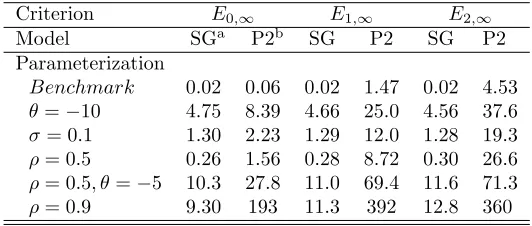
Table1shows that the maximal relative error for the benchmark parameteri-zation is three times larger for the approximation of the Taylor series expansion than for the semi-global method, however the errors for both these methods are very small - 0.06% and 0.02%, respectively. The increase in the condi-tional volatility of the rate of growth of dividends toσ= 0.1 yields the higher approximation errors of 2% and 1% for the local Taylor series expansion and semi-global method, respectively. Increasing the curvature of the utility func-tion to θ = −10 yields the maximal approximation error 8.4% for the Taylor series expansion approximation and about two times smaller for the semi-global method.

Table 1: The relative errors of the approximate solutions Criterion E0,∞ E1,∞ E2,∞

Model SGa _P2b _{SG P2 SG P2}

Parameterization

Benchmark 0.02 0.06 0.02 1.47 0.02 4.53

θ=−10 4.75 8.39 4.66 25.0 4.56 37.6

σ= 0.1 1.30 2.23 1.29 12.0 1.28 19.3

ρ= 0.5 0.26 1.56 0.28 8.72 0.30 26.6

ρ= 0.5, θ=−5 10.3 27.8 11.0 69.4 11.6 71.3

ρ= 0.9 9.30 193 11.3 392 12.8 360 a The semi-global method of order two

b The local Taylor series perturbation method of order two (Schmitt-Groh´e, and Uribe(2004))

andE2,∞. Furthermore, for any parameterization the semi-global

approxima-tion gives at least 5 times more accurate soluapproxima-tion in the metrics E1,∞ and 9

times in the metricsE2,∞than the local Taylor series expansion.

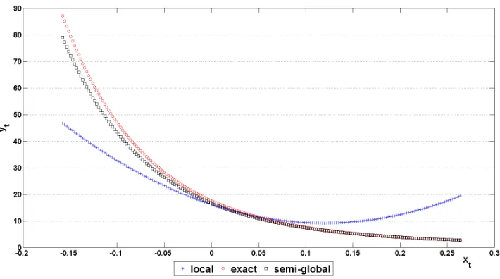
Figure 1 shows the policy functions for the high persistence case, ρ= 0.9, and indicates that the semi-global method traces globally the pattern of the true policy function much better than the local Taylor series expansion. More-over, from Figure 1 we can also see another undesirable property of the the local Taylor series expansion, namely this method can provide impulse response functions with a wrong sign. Indeed, the steady state value ofyt is ¯y = 12.3. After a positive shock the true impulse response function is negative, whereas the impulse response function implied by the local perturbation method is pos-itive, if the shock is large enough. Note also that the solution produced by the semi-global method is indistinguishable from the true solution for positive shocks (the bottom right corner of the Figure1).

7

Conclusion

This study proposes a method based on a perturbation around a deterministic path for constructing approximate solutions to DSGE models. The solutions obtained are global in the state space whenever so is the deterministic solution. As by product, an approach to solve linear rational expectations models with deterministic time-varying parameters is developed. This approach might be valuable in itself, for example, it can be used to solve Markov-Switching DSGE models. All results are obtained for DSGE models in general form and proved rigorously.

Figure 1: Comparison of the policy functions for ρ= 0.9.

modeling, such as projection and stochastic simulations, suffer from the curse of dimensionality, i.e. they can handle only small-dimension models. The pro-posed approach has a potential to solve high-dimensional models as it shares some preferable properties with the local perturbation methods. Namely, the computational gain may come from calculation of conditional expectations. To compute the conditional expectations using the semi-global method all that we need is to know the moments of the distribution up to the order of approxi-mation, while the use of the global methods mentioned above involves either stochastic simulations or quadratures. The former is time consuming, the later can deal with only low-order integrals. The practical implementation of the approach to larger size models the author leaves for future research.

A

Proofs for Section

5

PROOF OF PROPOSITION5.1: The proof is by induction oni. Suppose that

i= 0. For the timeT from (5.8) we have

ETuT+1=BT+1uT +Q21,T+1sT+ Ψ2,T+1ETηT+1.

AsBT+1 is invertible, we have

uT ,T =−KT ,TsT −gT ,0+L−T ,T,T1 ETuT+1,

where KT ,T = B−_T+11 Q21,T+1; gT ,0 = −B_T−₊₁1 Ψ2,T+1ETηT+1 and L−_{T ,T}1₊₁ =

proved fori= 0. Assuming that (5.11) holds fori >0, we will prove it fori+ 1. To this end, consider Equation (5.8) for the timet=T−i−1. As the matrix

BT−i is invertible, we obtain

uT ,T−i−1=−B_T−−1iQ21,T−isT−i−1−B_T−−1iΨ2,T−iET−i−1ηT−i+BT−−1iET−i−1uT ,T−i.

Substituting the induction assumption (5.11) foruT ,T−i yields uT ,T−i−1=−B_T−−1iQ21,T−isT−i−1−B

−1

T−iΨ2,T−iET−i−1ηT−i

+B_T−₋1_iET−i−1

h

−KT ,T−isT−i+gT ,i+

Qi+1

k=1L

−1

T ,T−i+k

ET−i(uT+1)

i

.

Substituting (5.7) forET−i−1(sT−i) and using the law of iterated expectations

gives

uT ,T−i−1=−BT−−1iQ21,T−isT−i−1−BT−−1iΨ2,T−iET−i−1ηT−i+BT−−1igT ,i

+B_T−₋1_iQi+1

k=1L

−1

T ,T−i+k

ET−i−1(uT+1)

+B_T−−1i[−KT ,T−i(AT−isT−i−1+Q12,T−iuT ,T−i−1+ Ψ1,T−iET−i−1ηT−i)].

Collecting the terms withuT ,T−i−1,sT−i−1andηT−i, we get

I+B_T−₋1_iKT ,T−iQ12,T−i

uT ,T−i−1=−BT−−1i

(Q21,T−i+KT ,T−iAT−i)sT−i−1

+(Ψ2,T−i+KT ,T−iΨ1,T−i)ET−i−1ηT−i+gT ,i+

Qi+1

k=1L

−1

T ,T−i+k

ET−i−1(uT+1)

Suppose for the moment that the matrixZT ,T−i =I+BT−−1iKT ,T−iQ12,T−i is

invertible. Pre-multiplying the last equation byZ_{T ,T}−1_−i, we obtain

uT ,T−i−1=−ZT ,T−1−iB

−1

T−i

(Q21,T−i+KT ,T−iAT−i)sT−i−1

+(Ψ2,T−i+KT ,T−iΨ1,T−i)ET−i−1ηT−i+gT ,i

+Qi+1

k=1L

−1

T ,T−i+k

ET−i−1(uT+1).

Note that LT ,T−i =BT−iZT ,T−i; then using the definition ofKT ,T−i−1 (5.9),

we see that

uT ,T−i−1=−KT ,T−i−1sT−i−1

−L−_{T ,T}1−i(Ψ2,T−i+KT ,T−iΨ1,T−i)ET−i−1ηT−i

+L−_{T ,T}1_−igT ,i+L−_{T ,T}1_−iQi+1

k=1L

−1

T ,T−i+k

ET−i−1(uT+1).

(A.1)

Using the definition ofgT ,iandLT−i,T−i+j ((5.10) and (5.12)), we deduce that gT ,i+1=−L−_{T ,T}1−i(Ψ2,T−i+KT ,T−iΨ1,T−i)ET−i−1ηT−i+L−T ,T1−igT ,i. (A.2)

From (A.1) and (A.2) it follows that

uT ,T−i−1=−KT ,T−i−1sT−i−1+gT ,i+1+

i+2

Y

k=1

L−_{T ,T}1_−i−1+k

!

This proves the proposition.

PROOF OF PROPOSITION5.2: We begin by rewriting (5.9) as

(BT−i+KT ,T−iQ12,T−i)KT ,T−(i+1)= (Q21,T−i+KT ,T−iAT−i).

Rearranging terms, we have

KT ,T−(i+1)=BT−−1i·(Q21,T−i+KT ,T−iAT−i)

−B_T−−1iKT ,T−iQ12,T−iKT ,T−(i+1).

(A.3)

Taking the norms and using the norm properties gives

K_{T ,T}−(i+1)

≤

B−_T−1_i

· kQ21,T−ik+

B_T−₋1_i

· kKT ,T−ik · kAT−ik

+ B_T−₋1_i

· kKT ,T−ik · kQ12,T−ik ·

KT ,T−(i+1)

.

Rearranging terms, we get

KT ,T_−(i+1)

≤

B−_T−1_i

· kQ21,T−ik+

B_T−₋1_i

· kKT ,T−ik · kAT−ik

1− B_T−₋1_i

· kKT ,T−ik · kQ12,T−ik

. (A.4)

Inequality (A.4) is a difference inequality with respect to kKT ,T−ik, i =

0,1, . . . , T, and with time-varying coefficientskAT−ik,

B−_T−1_i

, kQ12,T−ik and

kQ21,T−ik. In (A.4) we assume that

1− B_T−₋1_i

· kKT ,T−ik · kQ12,T−ik 6= 0.

This is obviously true if kKT ,T−ik = 0. We shall show that if the initial

condition kKT ,T+1k = 0, then 1−

B_T−₋1_i

· kKT ,T−ik · kQ12,T−ik > 0, i =

1,2, . . . , T. Indeed, consider the difference equation:

si+1=

bd+basi

(1−bcsi). (A.5)

Lemma A.1. If inequality (5.13)holds, then the difference equation (A.5)has two fixed points

s∗1=

2bd

1−ba+p

(1−ba)2_−4b2_cd, (A.6)

s∗

2=

1−ba+p

(1−ba)2_−4b2_cd

2bc ,

wheres∗

1 is a stable fixed point whereass∗2 is an unstable one. Moreover, under

the initial conditions0= 0the solutionsi, i= 1,2, . . . ,is an increasing sequence

and converges tos∗

1.

The lemma can be proved by direct calculation. From (5.4)–(5.3) the values

a,b,canddmajorizekAT−ik,

B_T−₋1_i

,kQ12,T−ikandkQ21,T−ik, respectively.

If we consider Equation (A.2) and inequality (A.5) as initial value problems with the initial conditions kKT ,T+1k = 0 and s0 = 0, then their solutions

words,kKT ,T−ik is majorized bysi. From the last inequality and LemmaA.1

it may be concluded that

kKT ,T−ik ≤s∗1, i= 0,1,2, . . . , T, T ∈N. (A.7)

From (A.6), (A.7) and (5.4) it follows that

B_T−₋1_i

· kKT ,T−ik · kQ12,T−ik ≤

2b2_dc

1−ba+p

(1−ba)2_−4b2_cd. (A.8)

From (5.13) we see that 2b2_{dc <(1−ab)}2_{/2. Substituting this inequality into}

(A.8) gives

B_T−₋1_i

· kKT ,T−ik · kQ12,T−ik ≤

(1−ba)2 2(1−ba+p

(1−ba)2_−4b2_cd)

< (1−ba)

2

2(1−ba)= 1−ba

2 <1,

(A.9)

where the last inequality follows from (5.6). This proves Proposition 2. PROOF OF PROPOSITION5.4: The assertion of the proposition is true if there exist constantsM andrsuch that 0< r <1 and for T ∈N

kKT ,j−KT+1,jk ≤M rT+1, j= 0,1,2, . . . . (A.10)

Note now that KT ,j (KT+1,j) is a solution to the matrix difference equation

(5.9) at i = T −j (i = T + 1−j) with the initial condition KT ,T+1 = 0

(KT+1,T+2= 0). Subtracting (A.3) forKT ,T−(i+1) from that forKT+1,T−(i+1),

we have

KT ,T−(i+1)−KT+1,T−(i+1)=BT−−1i(KT ,T−i)−KT+1,T−i)AT−i

−B_T−₋1_iKT ,T−i)Q12,T−iKT ,T−(i+1)+B−T−1iKT+1,T−iQ12,T−iKT+1,T−(i+1).

Adding and subtractingB−_T−1_i·KT ,T−i·Q12,T−i·KT+1,T−(i+1)in the right hand

side gives

KT ,T−(i+1)−KT+1,T−(i+1)=BT−−1i(KT ,T−i)−KT+1,T−i)AT−i

−B−_T−1_i·KT ,T−i·Q12,T−i(KT ,T−(i+1)−KT+1,T−(i+1))

−B−_T−1_i(KT ,T−i−KT+1,T−i)Q12,T−i·KT+1,T−(i+1).

Rearranging terms yields

(I+B_T−₋1_iKT ,T−iQ12,T−i)(KT ,T−(i+1)−KT+1,T−(i+1))

=B_T−₋1_i(KT ,T−i−KT+1,T−i)AT−i

−B_T−₋1_i(KT ,T−i−KT+1,T−i)Q12,T−iKT+1,T−(i+1).

From Proposition5.3it follows that the matrix

is invertible, then pre-multiplying the last equation by this matrix yields

KT ,T−(i+1)−KT+1,T−(i+1)=ZT ,T−1−i(B

−1

T−i(KT ,T−i−KT+1,T−i)AT−i

−B−_T−1_i(KT ,T−i)−KT+1,T−i)Q12,T−iKT+1,T−(i+1)).

Taking the norms, using the norm property and the triangle inequality, we get

kKT ,T−(i+1)−KT+1,T−(i+1)k

≤ kZ_{T ,T}−1−ik ·(kB

−1

T−ik · kKT ,T−i−KT+1,T−ik · kAT−ik

+kB−_T−1_ik · kKT ,T−i)−KT+1,T−ik · kQ12,T−ik · kKT+1,T−(i+1)k).

(A.11)

From (5.3) and (A.9) we have

kKT ,T−(i+1)−KT+1,T−(i+1)k

≤

ab+1−ba 2

kZ_{T ,T}−1_−ik · kKT ,T−i−KT+1,T−ik

= 1 +ba 2 kZ

−1

T ,T−ik · kKT ,T−i−KT+1,T−ik.

(A.12)

From the norm property and Golub, and Van Loan (1996, Lemma 2.3.3) we get the estimate

kZ_{T ,T}−1_−ik=k(I+B−_T−1_iKT ,T−iQ12,T−i)−1k ≤

1

1− kB−_T−1_iKT ,T−iQ12,T−ik

≤ 1

1− kB_T−₋1_ik · kKT ,T−ik · kQ12,T−ik

By (A.9), we have

kZ_{T ,T}−1_−ik=< 1

1−1−ba

2

= 2

1 +ba

Substituting the last inequality into (A.12) gives

kKT ,T−(i+1)−KT+1,T−(i+1)k<kKT ,T−i−KT+1,T−ik. (A.13)

Using (A.16) successively for i = −1,0,1, . . . , T −1, and taking into account

KT ,T+1= 0 andKT+1,T+1=B_T−+21 Q21,T+2 results in

kKT ,j−KT+1,jk<kKT ,T+1−KT+1,T+1k=kBT−+21 Q21,T+2k

≤ kB−_T+21 k · kQ21,T+2k ≤bkQ21,T+2k, j= 0,1,2, . . . .

(A.14)

Recall thatQ21,T depends on the solution to the deterministic problem (3.11),

i.e. Q21,T =Q21

x(0)_T+1, x(0)_T , z(0)_T+1, z(0)_T . FromHartmann(1982, Corollary 5.1) and differentiability ofQ21 with respect to the state variables it follows that

whereαis the largest eigenvalue modulus of the matrixAfrom (4.6),Cis some constant andθis arbitrary small positive number. In fact,α+θdetermines the speed of convergence for the deterministic solution to the steady state. Inserting (A.15) into (A.16), we can conclude

kKT ,j−KT+1,jk< bC(α+θ)T+2, j= 0,1,2, . . . (A.16)

DenotingM =bC(α+θ) and r=α+θ we finally obtain (A.10). This proves the proposition.

B

Series expansion for Burnside’s model

Substituting (6.5) and (6.6) into (6.2) yields

y(0)_x(0)

t +σx

(1)

t

+σy(1)_x(0)

t +σx

(1)

t

+σ2_y(2)_x(0)

t +σx

(1)

t

+· · ·

=βEt

exphθx(0)_t+1+σx(1)_t+1i

1 +y(0)x(0)_t+1+σx(1)_t+1+σy(1)x(0)_t +σx(1)_t

+σ2y(2)x(0)_t+1+σx(1)_t+1+· · ·

Expandingyt for smallσup to order two gives

y(0)_t +σy₁(0)_,tx(1)_t +1 2σ

2_y(0) 2,t

x(1)_t 2+σy(1)x(0)_t +σ2y₁(1)_,tx(1)_t +σ2y(2)_t +· · ·

=βEtexp(θx(0)_t+1)

1 +σθx(1)_t+1+1 2

σθx(1)_t+12+· · ·

1 +y_t(0)₊₁+σy(0)_1,t+1x(1)_t+1

+σ21

2y

(0) 2,t+1

x(1)t+1

2

+σyt(1)+1+σ2y (1) 1,t+1x

(1)

t+1+σ2y (2)

t+1+· · ·

Collecting the terms of like powers ofσof the last equation, we have

yt(0)+σ

h

(y(0)1,tx

(1)

t +y(1)x

(0)

t

i

+σ2

y(2)+y(1)2,tx

(1) t + 1 2y (0) 2,t

x(1)t

2

+· · ·

=βexpθx(0)_t+1

Et

(1 +y(0)_t+1) +σ

h

θx(1)_t+1(1 +y (0)

t+1) +y (0) 1,t+1x

(1)

t+1+y (1)

t+1

i

+σ21

2(θx

(1)

t+1)2(1 +y (0)

t+1) +y (2)

t+1+y (1)

t+1x (1)

t+1+y (1) 1,t+1x

(1)

t+1+

1 2y

(0) 2,t+1

x(1)_t+1

2

+θy₁(0)_,t+1x(1)_t+12+θx(1)_t+1y(1)_t+1

+· · ·

References

Adjemian, S., H. Bastani, M. Juillard, F. Karam´e, F. Mihoubi, G. Perendia, J. Pfeifer, M. Ratto, and S. Villemot (2011): “Dynare: Reference Manual, Version 4.” Dynare Working Papers, 1, CEPREMA

Anderson, G., andG. Moor(1985): “A Linear Algebraic Procedure for Solv-ing Linear Perfect Foresight Models,”Economics Letters 17247–252

Andreasen, M., J. Fern´andez-Villaverde, and J. F. Rubio-Ramrez(2013): “The Pruned State-Space System for Non-Linear DSGE Models: Theory and Empirical Applications,” NBER Working Paper No. 18983.

Blanchard, O.J., andC.M. Kahn(1980): “The Solution of Linear Difference Models Under Rational Expectations,” Econometrica 481305–1311.

Boroviˇcka, J., andL. P. Hansen (2013): “Examining Macroeconomic Mod-els through the Lens of Asset Pricing.” Working Paper

Burnside, C. (1998): ”Solving asset pricing models with Gaussian shocks,”

Journal of Economic Dynamics and Control 22 329–340

Collard, F., andM. Juillard(2001): “Accuracy of stochastic perturbation methods: the case of asset pricing models,”Journal of Economic Dynamics and Control 25979–999.

Den Haan, W. J., and J. De Wind (2012): “Nonlinear and stable perturbation-based approximations,” Journal of Economic Dynamics and Control 361477–1497.

Fair, R., andJ.Taylor(1983): “Solution and maximum likelihood estimation of dynamic rational expectation models,”Econometrica 511169–1185.

Gaspar, J. ,and K. L. Judd (1997): “Solving Large-Scale Rational-Expectations Models,”Macroeconomic Dynamics 145–75.

Golub, G.H., and C.F.Van Loan (1996): Matrix Computations, 3rd ed. Johns Hopkins University Press, Baltimore.

Gomme, P., andP. Klein(2011): “Second-Order Approximation of Dynamic Models without the Use of Tensors,” Journal of Economic Dynamics and Control 35604–615.

Hartmann, P. (1982): Ordinary Differential Equations, 2nd ed. Wiley, New York.

Holmes, M. H.(2013): Introduction to Perturbation Methods, 3rd ed Springer-Verlag, Berlin-Heidelberg-New-York-Tokyo.

Jin, H., and K. L. Judd(2002): “Perturbation methods for general dynamic stochastic models.” Discussion Paper, Hoover Institution, Stanford.

Judd, K. L.(1998): Numerical Methods in Economics, The MIT Press, Cam-bridge.

Judd K. L., and S.-M. Guu (1997): ”Asymptotic Methods for Aggregate Growth Models,”Journal of Economic Dynamics and Control211025–1042.

Juillard, M.(1996): “DYNARE: a program for the resolution and simulation of dynamic models with forward variables through the use of a relaxation algorithm.” CEPREMAP working paper No. 9602, Paris

Kim, J., S.Kim, E.Schaumburg, and C. A.Sims(2008): “Calculating and using second order accurate solutions of discrete time dynamic equilibrium models,”Journal of Economic Dynamics and Control 323397–3414.

Lombardo, G.(2010): “On Approximating DSGE Models by Series Expan-sions,” European Central Bank Working Paper Series, No. 1264.

Mehra, R., and E.C. Prescott(1985): “The equity premium: a puzzle,”

Journal of Monetary Economics 15145–161.

Schmitt-Groh´e, S., and M.Uribe (2004): “Solving dynamic general equi-librium models using as second-order approximation to the policy function,”

Journal of Economic Dynamics and Control 28755–775.

Sims, C.A.(2001): “Solving Linear Rational Expectations Models,” Computa-tional Economics 201–20.