Audio Visual Speech Recognition for People with Speech Disorders

Audio-Visual Speech Recognition for People with

Speech Disorders

Elham S. Salama

Information Cairo University

Reda A. El-Khoribi

Faculty of Computers and Information Cairo University

Mahmoud E. Shoman

Faculty of Computers and Information Cairo University

ABSTRACT

Speech recognition of disorder people is a difficult task due to the lack of motor-control of the speech articulators. Multimodal speech recognition can be used to enhance the robustness of disordered speech. This paper introduces an automatic speech recognition system for people with dysarthria speech disorder based on both speech and visual components. The Mel-Frequency Cepestral Coefficients (MFCC) is used as features representing the acoustic speech signal. For the visual counterpart, the Discrete Cosine Transform (DCT) Coefficients are extracted from the speaker's mouth region. Face and mouth regions are detected using the Viola-Jones algorithm. The acoustic and visual input features are then concatenated on one feature vector. Then, the Hidden Markov Model (HMM) classifier is applied on the combined feature vector of acoustic and visual components. The system is tested on isolated English words spoken by disorder speakers from UA-Speech data. Results of the proposed system indicate that visual features are highly effective and can improve the accuracy to reach 7.91% for speaker dependent experiments and 3% for speaker independent experiments.

General Terms

Audio-Visual Speech Recognition, Speech Disorder,

Dysarthria.

Keywords

AVSR, HMM, HTK, MFCC, DCT, UA-Speech, OpenCV.

1.

INTRODUCTION

Automatic speech recognition (ASR) is used in many assistive fields such as human computer interaction, and robotics. In spite of their effectiveness, speech recognition technologies still need more work for people having speech disorder. Because speech is not spoken in isolation, such that there are some visual movements of the lips, so, making use of visual features from the lip region can improve the accuracy compared to audio only ASR. Visual features are studied in many recent audio-visual ASR systems for normal speakers [1, 2].

In this paper, the effect of adding visual features on the performance of speech recognition system of disorder people compared to audio only speech recognition systems will be discussed. The interest of this paper is in speakers with dysarthria disorder type, one of the most known diseases in articulation disorder. Three different visual features selection methods are compared and the concentrate this work is on English isolated words.

The rest of this paper is organized as follows. Section 2 discusses previous related works. Section 3 explains the block diagram of the proposed system. The experimental results for normal and abnormal speakers are introduced in section 4. Section 5 contains a conclusion about what have been achieved through this research and future work.

2.

RELATED WORK

Dysarthria is a type of motor speech disorders where normal speech is disrupted due to loss of control of the articulators that produce speech [3]. Limited research studies for automatic recognition of speech disorders have been done previously. In [4], Authors described the results of experiments in building recognizers for talkers with spastic disorder using HMM. Authors in [5] presented an automatic speech recognition system of disorders in continuous speech using Artificial Neural Network (ANN) approach. Researchers in [6] reported that the speaker independent (SI) systems have low recognition accuracy for dysarthria speakers; so, speaker dependent (SD) systems have been investigated in some papers reporting that this system type is more suitable for disorder people than SI systems especially for severe cases of dysarthria speakers [6]. An SD system for disorder speakers based on HMM, Dynamic Bayesian networks (DBN) and Neural Networks was presented in [7]. As described, researches on automatic recognition of disordered speech have been focused on recognition of acoustic speech only whose performance degrades in the presence of ambient noise. However, visual features generated from the speaker's lip region have recently been proposed as an active modality to enhance normal speech recognition [1, 2]. The advantage of the visual-based speech recognition is that it is immune to background acoustic noise [8]. Also, human make use of visual signals to recognize speech [9, 10] and the visual modality has information that is related to audio modality [11].

The accuracies obtained by the above researches are reasonably high, but it is still needed to get further improvement for disorders. Next section describes the proposed system which uses the visual features to enhance the recognition accuracy.

3.

PROPOSED SYSTEM

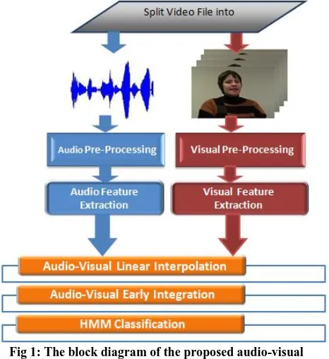
Figure 1 presents a typical audio-visual speech recognition system that is tested for disorder speakers. The input video that contains the speakers' spoken word is divided into audio file and its corresponding image files. There are two working threads, the audio front-end and images (visual) front-end. The audio-visual feature linear interpolation and integration processes are then performed. Finally, the HMM classification is applied to classify the words to their respective classes with the use of both audio and visual features.

Fig 1: The block diagram of the proposed audio-visual speech recognition system

3.1

Audio Front-End

In this sub-section, preprocessing steps done on the audio files and feature extraction are described.

3.1.1.

Audio Pre-Processing

Before extracting the acoustic features, there are required pre-processes that have to be done on the speech file. Essential preprocessing step is framing or segmentation, means dividing the speech signal into smaller pieces because speech signal is assumed to be stationary with constant statistical properties for small period of time typically 25 msec. this is done by cross-multiplying the signal by a window function which is zero everywhere except for the region of interest. Another process that has to be done to ensure the continuity of the speech signal is overlapping the speech signal with adjacent frames. The typical value for the frame overlap period is 10 msec.

3.1.2.

Audio Feature Extraction

The Mel-Frequency Cepestral Coefficients (MFCC) is chosen as one of the most common audio features [14]. MFCC is based on known variations of the bandwidth of the human ear

which cannot perceive frequencies over 1 KHz. Figure 2 shows the main steps in calculating MFCC. 13 MFCC features are extracted together with their 1st and 2nd derivatives producing an acoustic feature vector of length 39 elements.

Fig 2: Steps of calculating the MFCC features

3.2. Visual Front-End

The pre-processing on the images of the input video, and visual feature extraction are shown in Figure 3 and explained in below sub-sections.

Fig 3: Visual front-end steps, pre-processing and feature extraction processes

3.2.1.

Visual Pre-Processing

The visual features are extracted from mouth region; so, the mouth region needs to be prepared first for the next visual features extraction step. The applied preprocessing processes are briefly explained.

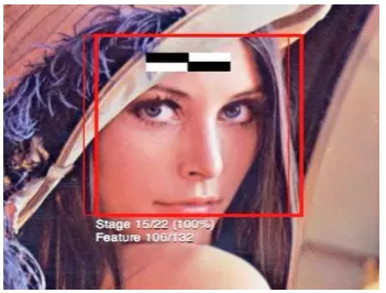
 Face Detection: In order to detect the mouth region, the face region is detected first in each frame in the video sequence. The Viola-Jones algorithm [15] is selected to achieve robust and real-time face detection. It is based on AdaBoost, a binary classifier that uses cascades of weak classifiers to boost its performance. Example of haar-like features is shown in Figure 4. It passes by many stages of applying the weak haar features on the face image to achieve a robust detection at the end. This step returns a rectangle around the detected face region.

 Mouth Detection: Again, the Viola-Jones algorithm is applied to detect the mouth from the above detected face region returning a rectangle around the mouth. This nested detection helps to minimizes the number of false positives in the image and subsequently increase the accuracy of mouth detection.

features be affected by the lip location in the input image. The chosen value of n to is 7 (128*128 pixels).

 Convert RGB to Gray: The input mouth image is of RGB format. It is converted to gray format in range 0 (black) to 255 (white).

Fig 4: Example of haar-like features (black and white rectangle) and how it applied for face detection (red

rectangles)

A simple output of each pre-processing step of visual front-end for an image from speaker M10 (from the used data in the proposed system) is shown in Figure 5.

Fig 5: Output of each visual pre-processing step. a) Face detected region. b) Mouth detected region. c) Mouth region only. d) Mouth region after resizing by 128*128.

and e) Mouth region as gray scale

To test the effectiveness of face and mouth detection using the Viola-Jones algorithm, 1900 random sample images from different speakers are selected and their face and mouth detection percentages are recorded. The percentage of detection reaches to 100% and 96.5% for face and mouth detection respectively.

3.2.2.

Visual Feature Extraction

There are two main visual feature extraction categories that are appearance or pixel based and shape or model based. Examples of model based features are the width and the height of the speaker's lips. There is a loss of information because it depends on some information about the lips not the whole region [16, 17]. Appearance based assumes that all mouth region pixels are informative to speech recognition [18, 19].

Examples of appearance-based features are DCT, Discrete Wavelet Transform (DWT), and Linear Discriminate Analysis (LDA).

Due to the good performance of the DCT in audiovisual speech recognition [2], it is applied in this study and extracted from speaker's mouth region. DCT outputs a matrix of features with the same dimension of the input mouth image file. Then, to calculate the final visual feature vector, three selection methods are applied.

 Method 1: Calculates the overall maximum values from the DCT matrix and append their 1st and 2nd derivatives. For Example, if 3 maximums are chosen, so the feature vector contains 3 maximums, their 3 1st derivatives and their 3 2nd derivatives. This produces visual feature vector with length of 9 elements.

 Method 2: Gets the upper left corner region of the DCT matrix. Say that dimension of this region is set to 3, so the region will be of size 3*3 and the final feature vector will be 9 elements.

 Method 3: The same as the second method but works only on maximum features not the whole upper left corner region. Example of that, if the dimension is 4 (4*4) and maximum is 3; so, the final vector will be 3 elements only.

After applying one of the above three method, the final visual feature is obtained. Figure 5 shows the above process of extracting the final visual feature vector.

3.3.Audio-Visual Features Integration

The features from different modalities (audio and visual features) have to be fused at some time. There are two different strategies to work with different type of features, early integration and late integration. In early integration (or what is called feature fusion), features from different sources are concatenated in one feature vector. The recognition process is applied on the combined feature vector. Late integration uses different or same classifiers for each feature type, and then the results of the classifiers are combined to get the final classification result.

In this study, early integration strategy by concatenating the acoustic and visual feature vectors on one vector is applied. However, the audio and visual are with different frame rates, 44.1 KHz and 30 Hz for audio and video respectively, so linear interpolation is required first to up sample the video features rate to be with the same frame rate as audio features

3.2.

HMM Classification

Hidden Markov Models (HMM) [20, 21] is proven to be a high reliable classifier for speech recognition applications for automatic speech recognition for normal and disorder people [4, 6]. HMM is applied on the combined vector of audio and visual features. In this study, a total of 10 HMM models, one for each word, are trained, and 45 phonemes are used to build each word's model. The number of states is determined experimentally with 3-Gaussian mixtures for each state.

4.

EXPERIMENTAL RESULT

4.1. Data Description

This database consists of 5 tasks of connected words produced by disorder individuals with cerebral palsy. The tasks are 10 digits ('Zero' to 'Nine'), 26 alphabet words (e.g. 'Echo', 'Sierra', 'Bravo'), 19 computer commands (e.g. 'Delete', 'Enter', 'Cut'), 100 common words (e.g. 'The', 'It', 'In') and 100 uncommon words (e.g. 'Naturalization', 'Frugality'). Each task is repeated 3 times per speaker.

UA-Speech contains speakers with large range of intelligibility (very low- low- mid - high) and each speaker has label representing male or female; speaker label starting by M is for male and F for female.

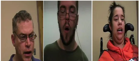
The standard resolution is 720 * 480 pixels for videos and a sampling frequency of 44.1 kHz for audio files. Sample images from the UA-Speech data can be seen in Figure 6.

Fig 6: Sample images from the UA-Speech Data, from left to right, M14, M16, and F04

Due to the way UA-Speech is recorded, data are segmented manually allowing about 0.1 silence boundary around each word to produce isolated word models.

4.2. System Configurations

To build the proposed AVSR system, there is need to specify the method by which we calculate the final visual feature vector. Table 1 lists the configurations of the tested methods and their parameters of maximum and dimension of upper left corner region. Changing the values of these parameters, seven configuration systems are tested. For configurations from C10 to C11, the final visual features are obtained from method 1 of DCT, while the configurations from C20 to C21 are obtained from method 2 of DCT. The visual features obtained from method 3 of DCT are in configurations from C30 through C32.

The values of parameters of each DCT method are indicated in Table 1 and the final length of the visual features for each configuration is also shown. As can be noticed, small values of visual feature vector are tested; range from 3 to 9 values. Hidden Markov Model Toolkit (HTK) [22] is used for training and testing the proposed ASR and AVSR. HTK has list of command line functions that perform the basic components of ASR. Also, HTK is used for extracting audio features. It extracts 13 MFCC features together with their 1st and 2nd _{derivatives producing an acoustic feature vector of} length 39 elements.

The applied tool for the face and mouth detection by Viola-Jones is OpenCV. OpenCV is an open source tool aimed at real-time computer vision [23]. It has tools for object detection using cascade of boosted classifiers working with haar-like features that is trained with a few hundred sample views of a particular object.

In order to discuss the effect of adding the DCT visual features on disorder data, two experiments are performed. Descriptions of each experiment and its obtained results are presented in the next section.

Table 1. The proposed AVSR system configurations

System Type

DCT Parameters Final

Visual Feature

Length Dimension

Number of Maximums

C10 ـــــــ 2 6

C11 ـــــــ 3 9

C20 2 ـــــــ 4

C21 3 ـــــــ 9

C30 3 3 3

C31 3 5 5

C32 3 7 7

4.3. Experiments

4.3.1.

Experiment 1: speaker dependent speech

recognition using acoustic and visual

features

In this experiment, speaker dependent (SD) models are generated for the disorder speakers by making use of speaker's data to train and test models for each disorder speaker dependently. The number of speakers used in this experiment is 5 speakers whose labels are F04, M06, M10, M14, and M16. Only the first 4 tasks from UA-Speech are used (digits, alphabet words, computer commands and common words) producing a set of 155 words. The total number of words in this experiment is 2,325 words (155 words from 4 tasks, each with 3 repetitions and 5 speakers). Blocks 1 and 2 of repetitions are used for training and block 3 is used for testing. The intelligibility of speakers ranges from 39%(M06-low) to 93% (M10-high). This experiment contains one female and four males.

The results of this experiment are shown in Table 2. Speakers are sorted according to their intelligibility which appears beside each speaker's label. The values appears in the row of each speaker are the ASR average accuracy for that speaker over the four tasks. Gray cells refer to the increase of accuracy occurs after adding visual features.

Another big note that can be found is that the increase of accuracy after adding visual features is affected by speaker's intelligibility, such that speakers with high intelligibility have large increase from all methods while low intelligibility speakers have small increase of accuracy. This can be shown from speakers M10 and M14 whose accuracy increases greatly compared to other speakers as they are the speaker with the highest intelligibility.

4.3.2.

Experiment 2: speaker independent

speech recognition using acoustic and

visual features

In this experiment, speaker independent (SI) manner is tried such that the data of all speakers appear both in training and testing phases. Testing is done using data from several speakers not only one speaker.

Ten speakers are used and their labels are F02, F04, F05, M05, M06, M08, M09, M10, M14 and M16. The speakers' intelligibility ranges from 29% (F02-low) to 95% (F05-high).

This experiment contains three females and seven males. The used task here is the digits task producing a total of 300 words (10 digits, 3 repetitions, and 10 speakers). 200 samples are used for training and 100 samples are used in testing.

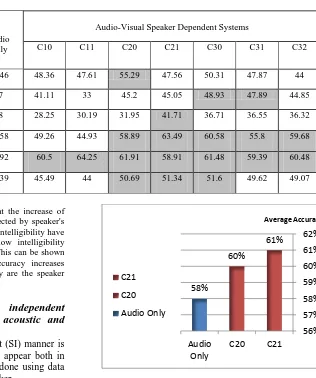
All the DCT configuration systems tried in above experiment are tried again here and the second method of DCT is the one that gets the best accuracy. The results of this experiment can be seen in Figure 7. An increase between 2% (using dimension 2) to 3% (using dimension 3) is achieved.

The most important advantage of the proposed system is that it depends on both the speech signal features and the DCT visual features from the speaker's mouth regions to improve the accuracy of speech disorder people.

Fig 7: Speaker independent audio and audio-visual accuracies of 10 speakers. Visual Results are using the 2nd

DCT feature selection method

4.

CONCLUSION

This study investigates the effect of adding Discrete Cosine Transform Coefficients of mouth region as visual features for disorder people with the audio features. The proposed system is tested on the standard speech disorder database; UA-Speech data. Speaker dependent and speaker independent experiments are tested and three DCT visual selection methods are applied and compared. It was found that adding the whole upper left corner region of DCT coefficients matrix can improve the performance of AVSR for disorders in speaker dependent and speaker independent cases. The increase of accuracy after adding visual features can reach to 7% in speaker dependent system and 3% for the speaker independent system.

Future work can be done by apply the Map-Adaptation techniques to enhance audio accuracy of disorders and further see the effectiveness of the proposed system.

ACKNOWLEDGMENT

We appreciate the Mark Hasegawa-Johnson’s group which allows us to work on their UA-Speech data of disorders. Also, we have a great appreciation to the Open Sources OpenCV and HTK tools.

61% 60%

58%

56% 57% 58% 59% 60% 61% 62%

C21 C20

Audio Only

Average Accuracy

C21

C20

Audio Only

Table 2. Speaker dependent speech recognition systems using audio features only and both audio and visual features

Audio-Visual Speaker Dependent Systems Audio

Only Speaker

Intelligibility

C32 C31

C30 C21

C20 C11

C10

44 47.87

50.31 47.56

55.29 47.61

48.36 53.46

M06 (39%) Low

44.85 47.89

48.93 45.05

45.2 33

41.11 47

M16 (43%)

36.32 36.55

36.71 41.71

31.95 30.19

28.25 38

F04 (62%) Mid

59.68 55.8

60.58 63.49

58.89 44.93

49.26 55.58

M14 (90.4%) High

60.48 59.39

61.48 58.91

61.91 64.25

60.5 57.92

M10(93%)

49.07 49.62

51.6 51.34

50.69 44

45.49 50.39

REFERENCES

[1] A.N. Mishra, Mahesh Chandra, Astik Biswas, and S.N. Sharan. 2013. Hindi phoneme-viseme recognition from continuous speech. International Journal of Signal and Imaging Systems Engineering (IJSISE).

[2] Estellers, Virginia, Thiran, and Jean-Philippe. 2012. Multi-pose lipreading and audio-visual speech recognition. EURASIP Journal on Advances in Signal Processing.

[3] H. Kim, M. Hasegawa-Johnson, A. Perlman, J. Gunderson, T. Huang, K. Watkin, and S. Frame. 2008. Dysarthric speech database for universal access research. In Proceedings of Interspeech. Brisbane. Australia. [4] H. V. Sharma and M. Hasegawa-Johnson. 2010. State

transition interpolation and map adaptation for hmm-based dysarthric speech recognition. NAACL HLT Workshop on Speech and Language Processing for Assistive Technologies (SLPAT).

[5] G. Jayaram and K. Abdelhamied. 1995. Experiments in dysarthric speech recognition using artificial neural networks. Journal of rehabilitation research and development.

[6] Heidi Christensen, Stuart Cunningham, Charles Fox, Phil Green, and Thomas Hain. 2012. A comparative study of adaptive, automatic recognition of disordered speech. INTERSPEECH. ISCA.

[7] F. Rudzicz. 2011. Production knowledge in the recognition of dysarthric speech. Ph.D. thesis. University of Toronto. Department of Computer Science.

[8] Potamianos G., Neti C., Luettin J., and Matthews I. 2004. Audio-visual automatic speech recognition: an overview. Issues in Visual and Audio-Visual Speech Processing. MIT Press Cambridge. MA.

[9] H. McGurk and J.W. MacDonald. 1976. Hearing lips and seeing voices. Nature.

[10]A.Q. Summerfield. 1987. Some preliminaries to a comprehensive account of audio-visual speech perception. In Hearing by eye. The psychology of lip-reading.

[11]Massaro DW., and Stork DG. 1998. Speech recognition and sensory integration. American Scientist.

[12]Chikoto Miyamoto, Yuto Komai, Tetsuya Takiguchi, Yasuo Ariki, and Ichao Li. 2010. Multimodal speech

recognition of a person with articulation disorders using AAM and MAF. In proceeding of Multimedia Signal Processing (MMSP).

[13] Ahmed Farag, Mohamed El Adawy, and Ahmed Ismail. 2013. A robust speech disorders correction system for Arabic language using visual speech recognition. Biomedical Research.

[14] Davis, S. B., and Mermelstein, P. 1980. Comparison of parametric representations for monosyllabic word recognition in continuously spoken sentences. IEEE Transactions on Acoustics, Speech and Signal Processing, (ASSP).

[15] Paul Viola and Michael J. Jones. 2001. Rapid Object Detection using a Boosted Cascade of Simple Features. IEEE CVPR.

[16] G. Potamianos, C. Neti, G. Gravier, A. Garg, and A.W. Senior. 2003. Recent advances in the automatic recognition of audiovisual speech.

[17] Potamianos G., Graf HP., and Cosatto E. 1998. An image transform approach for HMM based automatic lipreading. In IEEE International Conference on Image Processing.

[18] Scanlon P, Ellis D, and Reilly R. 2003. Using mutual information to design class specific phone recognizers. In Proceedings of Eurospeech.

[19] P. Scanlon and G. Potamianos. 2005. Exploiting lower face symmetry in appearance-based automatic speechreading. Proc. Works. Audio-Visual Speech Process. (AVSP).

[20] Rabiner, L. 1989. A tutorial on hidden Markov models and selected applications in speech recognition. Proceedings of the IEEE.

[21] Tian, Y., Zhou, J.L., Lin, H., and Jiang, H. 2006. Tree-Based Covariance Modeling of Hidden Markov Models. IEEE transactions on Audio, Speech and Language Processing.

[22] S. Young, D. Kershaw, J. Odell, V. Valtchev, and P . Woodland. 2006. The HTK Book Version 3.4. Cambridge University Press.

[23] 2013. The OpenCV Reference Manual. Release

2.4.6.0. [Online]. Available: