Implementation and Comparative Study of Algorithms to
Avoid Obstacles in Mobile Robot Navigation
Min Raj Nepali
Final year, Bachelors, Department of EEE
Nitte Meenakshi Institute of Technology,
Bangalore
Amar Mani Aryal
Final year, Bachelors, Department of ECE
Nitte Meenakshi Institute of Technology,
Bangalore
Ashutosh
Final year, Bachelors, Department of ECE
Nitte Meenakshi Institute of Technology,
Bangalore
Kamal
Lamichhane
Final year, Bachelors, Department of ECE
Nitte Meenakshi Institute of Technology,
Bangalore
ABSTRACT
It is a challenging task to make a mobile robot navigate to a desired goal in an environment with obstacles. It is sure that, just path planning algorithm will not be able to guide the robot to the desired goal in such environment. Certain kind of Obstacle avoiding algorithm is to be incorporated along with the path planning algorithm to achieve the aforementioned objective. Among the various existing algorithms an attempt to implement Bug algorithm and Virtual goal algorithm and the comparative study on the same was done. Numbers of experiments were conducted to draw the inference that, which algorithm is better. To conduct the experiments the algorithms were run in NXPLPC 1768 microcontroller. For detecting the Obstacles the system was equipped with a ring of eight sonar. For simulation MATLAB was used. The conclusion that, virtual goal method is better than the bug algorithm is drawn finally through number of experiments and observations.
Keywords
Autonomous Mobile robots, Robot navigation, Obstacle avoidance, Nonlinear control systems.
1. INTRODUCTION
When a mobile robot navigates towards a goal, it is supposed to avoid obstacles lying in its path of motion. The robot should evaluate the distance to the goal as well as distance of the obstacle. Hence, the robot should know the goal coordinates and orientation. Thus the objective is to frame the robot movement such that the difference between goal position and the current position of the robot is minimum, leaving all the obstacles behind and respecting to the orientation.
Many approaches have been proposed to guide the robot to accomplish such task. Some of them use already known map of the environment to deduce path for robot navigation, also called as global path planning. In such condition, from the known map of the surrounding environment, the control algorithm plans the motion model to achieve the desired task. Other approaches to avoid that obstacles are based on the fact that no such known map or prior information about the surrounding environment is available but still robot should be able to navigate towards the goal by suitably reacting with the environment. To know about the environment, the system demands suitable sensing unit. On employing this method, any changes in the environment can be easily adjusted.
2. PLATFRORM OVERVIEW AND
SPECIFICATIONS
[image:1.595.330.549.448.612.2]The present work makes use of mbed NXPLPC1768 to realize the proposed algorithms. The Microcontroller in particular is designed for prototyping all sorts of devices, especially those including Ethernet, USB, and the flexibility of lots of peripheral interfaces and FLASH memory. It is packaged as a small DIP form-factor for prototyping with through-hole PCBs, strip board and breadboard, and includes a built-in USB FLASH programmer. The board has features like 96MHz clock , 32KB RAM, 512KB FLASH, Ethernet, USB Host/Device, 2xSPI, 2xI2C, 3xUART, CAN, 6xPWM, 6xADC, GPIO, etc. The board is equipped with High performance ARM® Cortex™-M3 Core.
Figure 1: MBED hardware.
3. NAVIGATING IN A FREE
ENVIRONMENT
SET THE GOAL
UPDATE ODOMETRY
GOAL REACHED?
YES NO START
[image:2.595.127.208.80.275.2]STOP
Figure 2: Flowchart showing the control process while navigating in free environment.
3.1 Representing Robot Position
Throughout the analysis the robot was modeled as a rigid body on wheels, operating on a horizontal plane. The robot chassis on the plane has total dimension is three, two for position in the plane and one for orientation along the vertical axis, which is orthogonal to the plane. Also, there are additional degrees of freedom and flexibility due to the, wheel steering joints, wheel castor joints and wheel axles. Here, robot chassis refers only to the unmovable body parts of the robot. Thus ignoring the joints and degrees of freedom internal to the robot and its wheels while considering robot chassis.
Figure 3: The global reference frame and the robot local reference frame.
In order to specify the position of the robot on the plane a relationship between the global reference frame of the plane and the local reference frame of the robot has been established, as in figure above. The axes X and Y define an arbitrary inertial basis on the plane as the global reference frame or the origin.
To specify the position of the robot, a point P on the robot chassis as its position reference point was chosen. The basis {x, y} defines two axes relative to P on the robot chassis and is thus the robot’s local reference frame. The position of the robot P in the global reference frame is specified by x-coordinate y-x-coordinate, and the difference in angle between
the global and local reference frames is given by θ. The robot pose can be described as a vector with these three elements.
XY
x
p = y (1) θ
To describe robot motion in terms of component motions, it will be necessary to map motion along the axes of the global reference frame to motion along the axes of the robot’s local reference frame. Obviously, this mapping is a function of the current pose of the robot. This mapping is accomplished using the orthogonal rotation matrix:
cosθ
sinθ 0
R(θ) = -sinθ cosθ 0 (2)
0
0
1
This matrix can be used to map motion in the global reference frame {x, y} to motion in terms of the local reference frame{x, y}. This operation is denoted by R(θ) Pxy because the computation of this operation depends on the value of θ:
xy XY
p = R(θ) p (3)
3.2 Kinematic Model
[image:2.595.94.236.452.577.2]The kinematics of the mobile robot captures how the robot moves, given its geometry and the speeds of its wheels. More formally, consider the example shown in figure below. This differential drive robot has two wheels, with radius rr and rl. Robot position reference point P centered between the two drive wheels, and distance between the wheels l. Given rr, rl, l, θ and the spinning speed of each wheel, φr and φl, a forward kinematic model would predict the robot’s overall speed in the global reference frame.
Figure 4: A differential-drive robot in its global reference frame.
XY r l r l
x
p = y = f l, r , r , θ, φ , φ (4) θ
From the above equation it is known that the robot’s motion can be computed in the global reference frame from motion in its local reference frame:
-1 XY xy
p = R(θ) p (5)
[image:2.595.323.531.466.580.2]robot’s local reference frame is aligned such that the robot moves forward along+x, as shown in figure. First consider the contribution of each wheel’s spinning speed to the translation speed at Pin the direction of+x. If one wheel spins while the other wheel contributes nothing and is stationary, since Pis halfway between the two wheels, it will move instantaneously with half the speed:
r r r
x = 1/ 2 r φ
l l l
x = 1/ 2 r φ
In a differential drive robot, these two contributions can simply be added to calculate the ẋ component of Ṗxy. Consider, for example, a differential robot in which each wheel spins with equal speed but in opposite directions. The result is a stationary, turning robot which turns about zero centre of rotation. As expected, ẋ will be zero in this case. The value of is ẏ even simpler to calculate. Neither wheel can contribute to sideways motion in the robot’s reference frame, nor so ẏ is always zero. Finally, it is required to compute the rotational component θ of Ṗxy. Once again, the contributions of each wheel can be computed independently and just added. Consider the right wheel (call this wheel 1). Forward gyration of this wheel results in counter-clockwise rotation at pointP. Recall that if the right wheel spins alone, the robot pivots around the left wheel. The rotation velocity ωr at P can be computed because the wheel is instantaneously moving along the arc of a circle of radius2l:
r r r
r φ ω =
2l
The same calculation applies to the left wheel, with the exception that forward gyration results in clockwise rotation at point P:
l l l
r φ ω =
2l
Combining these individual formulas yields a kinematic model for the differential-drive robot:
r φ + r φ
r r l l
2 -1
p = R θ 0 (6)
XY
r φ - r φ
r r l l
2l
3.3 Motion Model
Generally the pose (position) of a robot at any time instant k is represented by the vector
x
p k = y (7) θ
For a differential-drive robot the position can be estimated starting from a known position by integrating the movement (summing the incremental travel distances). For a non-continuous (discrete) system with a fixed sampling interval Δt the incremental travel distances (Δx;Δy;Δθ) are:
Δx = Δscos θ + Δθ / 2
Δy = Δssin θ + Δθ / 2
r l
Δs - Δs Δθ =
l
r l
Δs + Δs Δs =
2 Where,
Δx;Δy;Δθ =
Distance traveled in the last sampling interval.
Δs ;Δs =r l
Distance travelled for the right and left wheelrespectively.
Thus the updated position
Δscos θ + Δθ / 2 x Δscos θ + Δθ / 2
p k +1 = p k + Δssin θ + Δθ / 2 = y + Δssin θ + Δθ / 2 (8)
Δθ θ Δθ
By using the relation for Δsand Δθ , the basic equation for Odometric position update (for differential drive robots) can further be obtained as:
r l r l
r l r l
r l
Δs + Δs Δs - Δs
cos θ +
2 l
x
Δs + Δs Δs - Δs
p k +1 = y + sin θ + (9)
2 l
θ
Δs - Δs l
As discussed earlier, Odometric position updates can give only a very rough estimate of the actual position. Due to integration errors of the uncertainties of p(k) and the motion errors during the incremental motion(ΔSr ,ΔSl), the position error based on odometry integration grows with time.
In the next step an error model for the integrated position p(k +1)will be established to obtain the covariance matrix of the Odometric position estimate P(k +1) . To do so, it is assumed that at the starting point the initial covariance matrix
P(k) is known. For the motion increment
Δs ;Δsr l
the following covariance matrix Q is assumed
r rr l
l l
k Δs 0
Q = cov Δs , Δs = (10)
0 k Δs
Where Kr and Kl are error constants representing the non-deterministic parameters of the motor drive and the wheel-floor interaction. As you can see, in the above equation following assumptions were made:
The two errors of the individually driven wheels are independent.
The variance of the errors (left and right wheels) is proportional to the absolute value of the travelled distances.
These assumptions, while not perfect, are suitable and will thus be used for the further development of the error model. The motion errorsare due to imprecise movement because of deformation of wheel, slippage, unequal floor, errors in encoders, and so on. The values for the error constants
r
k an
k
l depend on the robot and the environment and should be experimentally established by performing and analyzing representative movements.by the first-order Taylor expansion (linearization), it is concluded, using the error propagation law:
T
T
p p q q
P k +1 = F k × P k × F k + F k ×Q× F k (11)
p
1 0 -Δssin θ + Δθ / 2
p p p
F k = = 0 1 Δscos θ + Δθ / 2 (12)
x y θ
0 0 1
Once the error model has been established, the error parameters must be specified. One can compensate for deterministic errors properly calibrating the robot. However the error parameters specifying the nondeterministic errors can only be quantified by statistical (repetitive) measurements.
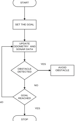
4. BUG ALGORITHM
[image:4.595.65.267.335.429.2]Obstacle avoidance is an indispensable behavior in mobile robots. If a robot does not contain sensors in it, it’s a blind robot. It keeps hitting whatever comes in its way.
Figure 5: Schematic of bug algorithm.
When the robot starts moving towards the goal it tries to reduce the distance between the goal position and its current position as well as simultaneously scans to find if any obstacle is present in its path [5-7].
SET THE GOAL
UPDATE ODOMETRY AND
SONAR DATA
OBSTACLE DETECTED
YES
NO START
STOP GOAL REACHED
AVOID OBSTACLE
NO
YES
Figure 6: Flowchart showing process flow of bug algorithm
When the robot reaches the point O it finds the obstacle is present in its path and the distance of the obstacle (dobs) from the robot as well. A threshold distance (dth) is defined such that if any obstacle is present within this distance, the robot is supposed to avoid the obstacle [1-3].Bug algorithm guides the robot as shown in the figure above. When the robot reaches the point O, it tries to change its path in order to avoid the obstacle. While doing so the robot follows the path generated by bug algorithm [4-5]. It can be seen that, when robot reaches point O it can either take right or left turn which is decided by the user. Suppose, the robot is programmed to take left, then the robot heads towards point P taking path 1. When following the path OP, the robot also calculates the difference between the goal position and its current position. At point P, the robot escapes the obstacle and heads towards the goal again.
Although the robot avoids the obstacle, it cannot avoid obstacles with corners (case of local minima) [3-6]. In such cases the robot gets stuck and never reaches the goal. To avoid such situation Virtual goal method is chosen.
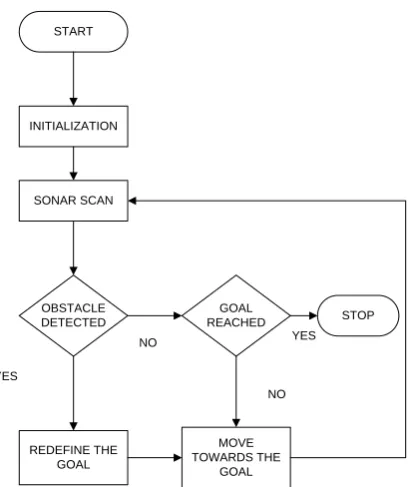
5. VIRTUAL GOAL METHOD
[image:4.595.322.522.495.595.2]The controller implemented to guide the robot while avoiding obstacles is nonlinear in nature. This algorithm has the capability to make the robot to avoid local minima also. A new goal position is generated whenever an obstacle is detected at a distance smaller than or equal to dobs from the robot [6-7]. Thus, distance between robot and the obstacle (dobs) defines the obstacle avoidance zone shown in Figure (6), and when the robot enters such a zone it should start moving away from that zone. Also, dmin is the smallest distance to be maintained between robot and obstacle, correspondent to a certain range scan. In the presence of an obstacle d min < dobsa temporary goal, Xv , known as virtual goal is created, whose position can be obtained on the basis of position of the real goal, Xd , with the help of a rotation matrix. It can be observed that the line connecting the point being controlled and the virtual goal is nearly tangent to the border of the detected obstacle, as shown in Figure (6).
Figure 7: Schematic for Virtual goal method
[image:4.595.67.210.499.730.2]γ ββ ββ
Notice that in Figure (6) , the angle γ is positive, causing the rotation of the real goal to the left, considering the axis of movement of the robot. As the robot navigates in a plane, the angle γ is used to get
γγ γγ
Where Xd and Xv are, respectively, the position of the real goal (desired) and the virtual goal. Having the coordinates of
Xv the position controller guides the robot to the new goal, following the tangent to the obstacle border. Notice that in the absence of obstacles there is no change in the position of the real goal (γ= 0), and the robot continues getting closer to the real goal [10-13]. The designer just has to define the distance dobs that characterizes the obstacle avoidance zone shown in Figure. Here in this experiment dobs was defined as 30 centimeter. This is an important characteristic of the strategy here proposed, because the system based on imaginary forces may cause the robot to get stuck in certain situations [7-9].
INITIALIZATION START
SONAR SCAN
OBSTACLE DETECTED
GOAL REACHED
REDEFINE THE GOAL
MOVE TOWARDS THE
GOAL
STOP
YES
NO
NO YES
Figure 8: flow diagram of virtual goal method.
6. SIMULATION AND EXPERIMENTAL
RESULTS
Several simulation and experimental results are conducted on the above discussed algorithms to obtain detailed and comparative study between those aforementioned algorithms. The algorithms were run on embedded platform provided by ArmCortex called as NXPLPC1768. The system was equipped with a ring of eight sonar sensor which is capable of scanning around 180 degrees at one scan time.
[image:5.595.337.524.313.674.2]Figure 9:Experimental setup with 8 Sonar Ring.
Figure 10: Sonar ring
Figure 11: Plot of practical values in Matlab for Virtual Goal Method.
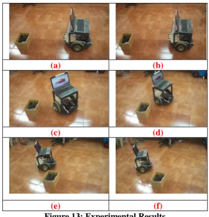
[image:5.595.67.273.315.559.2]Figure 13: Experimental Results
(a) (b)
(c) (d)
(e) (f)
From the above plots it can be observed that Bug algorithm cannot properly guide the robot, meaning the algorithm is being able to avoid the obstacle but the path is not proper. It can be clearly visualized that in Virtual goal method after the robot avoids the obstacle it has returned to the original path and then reached the goal which is a correct way of navigation since it has maintained its orientation as well. But that is not the case in bug algorithm where the robot reaches goal first and finally tries to orient itself.
7. CONCLUSION
A comparative study is carried out between Bug algorithm and Virtual goal method to avoid obstacle when a mobile robot is seeking a goal. From the above plots and experimental results it can be observed that Virtual goal method is dominant over Bug algorithm. Bug algorithm is just able to avoid obstacles but Virtual goal method is capable of even avoiding local minima meaning Virtual goal method does not let robot stuck around corner like objects. The virtual goal method and control system thus implemented is shown to be globally stable if there are no any obstacles present in the environment, and able to leave all obstacles behind. Therefore, the Virtual goal approach guarantees that the robot will reach any reachable goal.
Several simulations and experiments, were run using the above two algorithms, with range measurements provided by a ring of eight sonar. Their results have shown that the proposed controller is capable to guide the robot to the goal without colliding with any obstacle. But the Virtual goal algorithm facilitates to avoid local minima and guide the robot past obstacle whatever the shape and size of the obstacle and under any circumstances which Bug algorithm cannot. So, it can be concluded that Virtual goal algorithm is more reliable than Bug algorithm.
8. ACKNOWLEDGEMENTS
The authors express their sincere gratitude to Prof. N R Shetty, Director, Dr. H C Nagaraj, Principal and Prof. Dr. H. M. Ravi Kumar HOD Dept of EEE, Dr. Jharna Majumdar, Dean R&D HOD-CSE (PG) for their encouragement and support to undertake project at NMIT. The authors thank the Research associate team of NMIT led by Sandeep kumar Malu for continuous support for guiding and involvement in the project.
9. REFERENCES
[1] Iqbal, J., Islam, R.U., Khan, H.: Modeling and Analysis of a 6 DOF Robotic Arm Manipulator, Canadian Journal on Electrical and Electronics Engineering, vol. 3, no. 6, pp. 300-306 (2012)
[2] Islam, R.U., Iqbal, J., Manzoor, S., Khalid, A., Khan, S.: An autonomous image-guided robotic system simulating industrial applications, IEEE International Conference on System of Systems Engineering (SoSE), Italy, pp. 344-349 (2012)
[3] Iqbal, J., Nabi, R.U., Khan, A.A., Khan, H.: A Novel Track-Drive Mobile Robotic Framework for Conducting Projects on Robotics and Control Systems. Life Sci J, ISSN
[4] 1097-8135, vol. 10 (3), pp.130-137 (2013)
[5] Iqbal, J., Tahir, A., Islam, R.U., Nabi, R.U.: Challenges and Future Perspectives, IEEE International Conference on Applied Robotics for the Power Industry (CARPI), Switzerland, pp. 151-156 (2012)
[6] Keiji, N., Kushleyev, A., Daniel D. Lee.: Sensor Information Processing in Robot Competitions and Real World Robotic Challenges. Advanced Robotics vol. 26(14), pp. 1539-1554 (2012) 6. Zhu, Y., Zhang, T., Song, J., Li., X.: A New Hybrid Navigation Algorithm for Mobile Robots in Environments with Incomplete Knowledge, Knowledge-Based Systems vol. 27, pp. 302-313 (2012)
[7] Oussama Khatib. Real time obstacle avoidance for manipulators and mobile robots. The International Journal of Robotics Research, 5(1):90–98, 1986. [8] Yasushi Yagi, Hiroyuki Nagai, Kazumasa Yamazawa,
and Masahiko Yachida. Reactive visual navigation based on omnidirectional sensing ‐ path following and collision avoidance. Journal of Intelligent and Robotic Systems, 31(4):379–395, 2001.
[9] F. Belkhouche and B. Belkhouche. A method for robot navigation toward a moving goal with unknown maneuvers. Robotica, 23(6):709–720, 2005.
[10]Ahmed Benzerrouk, Lounis Adouane, and Philippe Martinet. Lyapunov global stability for reactive mobile robot navigation in presence of obstacles. In Proceedings of the ICRA10 Workshop on Robotics and Intelligent Transportation System, Alaska, USA, 2010.
[11]Krogh, B. H. and Thorpe, C. E., "Integrated Path Planning and Dynamic Steering Control for Autonomous Vehicles." Proceedings of the 1986 IEEE International Conference on Robotics and Automation, San Francisco, California, April 7-10, 1986, pp. 1664-1669.
[12] Moravec, H. P. and Elfes, A., "High Resolution Maps from Wide Angle Sonar." IEEE Conference on Robotics and Automation, Washington D.C., 1985, pp. 116-121. [13] Eilove, R. B., "Local Obstacle Avoidance for Mobile
Robots Based on the Method of Artificial Potentials." General Motors Research Laboratories, Research Publication GMR-6650, September 1989.
[14]Jun Zhou, Bolandhemmat. H, “Integrated INS/GPS System for an Autonomous Mobile Vehicle”, International Conference on Mechatronics and Automation, ICMA, pp. 694-699, 2007.