A Comparative Study on Numerical Solutions of Initial Value Problems (IVP) for Ordinary Differential Equations (ODE) with Euler and Runge Kutta Methods

(1)

http://dx.doi.org/10.4236/ajcm.2015.53034

A

Comparative

Study

on

Numerical

Solutions

of

Initial

Value

Problems

(IVP)

for

Ordinary

Differential

Equations

(ODE)

with

Euler

and

Runge

Kutta

Methods

Md.AmirulIslam

Department of Mathematics, Uttara University, Dhaka, Bangladesh

Email:

Received 17 August 2015; accepted 22 September 2015; published 25 September 2015

This work is licensed under the Creative Commons Attribution International License (CC BY).

Abstract

ThispapermainlypresentsEulermethodandfourth‐orderRungeKuttaMethod(RK4)forsolving initialvalueproblems(IVP)forordinarydifferentialequations(ODE).Thetwoproposedmethods arequiteefficientandpracticallywellsuitedforsolvingtheseproblems.Inordertoverifytheac‐ curacy,wecomparenumericalsolutionswiththeexactsolutions.Thenumericalsolutionsarein good agreement with the exact solutions. Numerical comparisons between Euler method and RungeKuttamethodhavebeenpresented.Alsowecomparetheperformanceandthe computa‐ tional effortof suchmethods. Inorder to achievehigher accuracyin the solution,the step size needstobeverysmall.Finallyweinvestigateandcomputetheerrorsofthetwoproposedmeth‐ odsfordifferentstepsizestoexaminesuperiority.Severalnumericalexamplesaregiventodem‐ onstratethereliabilityandefficiency.

Keywords

InitialValueProblem(IVP),EulerMethod,RungeKuttaMethod,ErrorAnalysis

1. Introduction

(2)

solve exactly, and one of two approaches is taken to approximate the solution. The first approach is to simplify the differential equation to one that can be solved exactly and then use the solution of the simplified equation to approximate the solution to the original equation. The other approach, which we will examine in this paper, uses methods for approximating the solution of original problem. This is the approach that is most commonly taken since the approximation methods give more accurate results and realistic error information. Numerical methods are generally used for solving mathematical problems that are formulated in science and engineering where it is difficult or even impossible to obtain exact solutions. Only a limited number of differential equations can be solved analytically. There are many analytical methods for finding the solution of ordinary differential equations. Even then there exist a large number of ordinary differential equations whose solutions cannot be obtained in closed form by using well-known analytical methods, where we have to use the numerical methods to get the approximate solution of a differential equation under the prescribed initial condition or conditions. There are many types of practical numerical methods for solving initial value problems for ordinary differential equations. In this paper we present two standard numerical methods Euler and Runge Kutta for solving initial value prob-lems of ordinary differential equations.

From the literature review we may realize that several works in numerical solutions of initial value problems using Euler method and Runge Kutta method have been carried out. Many authors have attempted to solve ini-tial value problems (IVP) to obtain high accuracy rapidly by using numerous methods, such as Euler method and Runge Kutta method, and also some other methods. In [1] the author discussed accuracy analysis of numerical solutions of initial value problems (IVP) for ordinary differential equations (ODE), and also in [2] the author discussed accurate solutions of initial value problems for ordinary differential equations with fourth-order Runge kutta method. [3] studied on some numerical methods for solving initial value problems in ordinary differential equations. [4]-[16] also studied numerical solutions of initial value problems for ordinary differential equations using various numerical methods. In this paper Euler method and Runge Kutta method are applied without any discretization, transformation or restrictive assumptions for solving ordinary differential equations in initial val-ue problems. The Euler method is traditionally the first numerical techniqval-ue. It is very simple to understand and geometrically easy to articulate but not very practical; the method has limited accuracy for more complicated functions.

A more robust and intricate numerical technique is the Runge Kutta method. This method is the most widely used one since it gives reliable starting values and is particularly suitable when the computation of higher de-rivatives is complicated. The numerical results are very encouraging. Finally, two examples of different kinds of ordinary differential equations are given to verify the proposed formulae. The results of each numerical example indicate that the convergence and error analysis which are discussed illustrate the efficiency of the methods. The use of Euler method to solve the differential equation numerically is less efficient since it requires h to be small for obtaining reasonable accuracy. It is one of the oldest numerical methods used for solving an ordinary initial value differential equation, where the solution will be obtained as a set of tabulated values of variables x and y. It is a simple and single step but a crude numerical method of solving first-order ODE, particularly suitable for quick programming because of their great simplicity, although their accuracy is not high. But in Runge Kutta method, the derivatives of higher order are not required and they are designed to give greater accuracy with the advantage of requiring only the functional values at some selected points on the sub-interval. Runge Kutta me-thod is a more general and improvised meme-thod as compared to that of the Euler meme-thod. We observe that in the Euler method excessively small step size converges to analytical solution. So, large number of computation is needed. In contrast, Runge Kutta method gives better results and it converges faster to analytical solution and has less iteration to get accuracy solution. This paper is organized as follows: Section 2: problem formulations; Section 3: error analysis; Section 4: numerical examples; Section 5: discussion of results; and the last section: the conclusion of the paper.

2. Problem

Formulation

In this section we consider two numerical methods for finding the approximate solutions of the initial value problem (IVP) of the first-order ordinary differential equation has the form

 









 

0

0 0

, , , _n

y f x y x x x x

y x y



   _



 _ (1)

(3)

paper we determine the solution of this equation on a finite interval



x x0, n



, starting with the initial point x0. A continuous approximation to the solution y x

 

will not be obtained; instead, approximations to y will be

generated at various values, called mesh points, in the interval



x x0, n



. Numerical methods employ the

Equa-tion (1) to obtain approximaEqua-tions to the values of the soluEqua-tion corresponding to various selected values of

0 , 1, 2,3, .

n

xx x nh n  The parameter h is called the step size. The numerical solutions of (1) is given by a set of points





x yn, n



:n0,1, 2, , n



and each point



x yn, n



is an approximation to the corresponding

point



x y xn,

 

n



on the solution curve.

2.1. Euler Method

Euler’s method is the simplest one-step method. It is basic explicit method for numerical integration of ordinary differential equations. Euler proposed his method for initial value problems (IVP) in 1768. It is first numerical method for solving IVP and serves to illustrate the concepts involved in the advanced methods. It is important to study because the error analysis is easier to understand. The general formula for Euler approximation is

 





1 , , 0,1, 2,3,

n n n n

y_ x  y x hf x y n .

2.2. Runge Kutta Method

This method was devised by two German mathematicians, Runge about 1894 and extended by Kutta a few years later. The Runge Kutta method is most popular because it is quite accurate, stable and easy to program. This method is distinguished by their order in the sense that they agree with Taylor’s series solution up to terms of

r

h where r is the order of the method. It do not demand prior computational of higher derivatives of y x

 

as

in Taylor’s series method. The fourth order Runge Kutta method (RK4) is widely used for solving initial value problems (IVP) for ordinary differential equation (ODE). The general formula for Runge Kutta approximation is

 





1 1 2 3 4

1

2 2 , 0,1, 2,3,

6

n n

y _ x  y x  k  k  k k n 

where

 

1 2





1 , , 2 ₂, ₂ , 3 ₂, ₂ , 4 , 3

k k

h h

k hf x y k hf x_  y _ k hf x_  y _ k hf xh yk

    .

3. Error

Analysis

There are two types of errors in numerical solution of ordinary differential equations. Round-off errors and Truncation errors occur when ordinary differential equations are solved numerically. Rounding errors originate from the fact that computers can only represent numbers using a fixed and limited number of significant figures. Thus, such numbers or cannot be represented exactly in computer memory. The discrepancy introduced by this limitation is call Round-off error. Truncation errors in numerical analysis arise when approximations are used to estimate some quantity. The accuracy of the solution will depend on how small we make the step size, h. A numerical method is said to be convergent if

 

0 1

lim max n n 0

h  n N y x y

  . Where y x

 

n denotes the approximate

solution and yn denotes the exact solution. In this paper we consider two initial value problems to verify

ac-curacy of the proposed methods. The Approximated solution is evaluated by using Mathematica software for two proposed numerical methods at different step size. The maximum error is defined by



 



1maxsteps

r n n

n

e y x y

 

  .

4. Numerical

Examples

In this section we consider two numerical examples to prove which numerical methods converge faster to ana-lytical solution. Numerical results and errors are computed and the outcomes are represented by graphically.

Example 1: we consider the initial value problem y x

 

x2xy, y

 

0 1 on the interval 0 x 1. The

exact solution of the given problem is given by

 

2 2

π

e erf e

2 2

x x

x

y x  _ _ x

  . The approximate results and

(4)

[image:4.595.88.539.133.721.2]

Table 1. (a) Numerical approximations and maximum errors for step size h0.1; (b) Numerical approximations and max-imum errors for step size h0.05; (c) Numerical approximations and maximum errors for step size h0.025; (d)

Nu-merical approximations and maximum errors for step size h0.0125.

(a)

Euler Method h0.1 Runge Kutta Method h0.1

n

x

 n

y x er y x n er

Exact Solution y_n

0.1 1.0000000000000000 5.34652E−03 1.0053464802083334 4.16045E−08 1.0053465218128410

0.2 1.0110000000000000 1.18895E−02 1.0228893798037348 8.26716E−08 1.0228894624752929

0.3 1.0352199999999998 1.99720E−02 1.0551918407370900 1.23029E−07 1.0551919637660336

0.4 1.0752765999999998 3.00424E−02 1.1053187896458685 1.63325E−07 1.1053189529706604

0.5 1.1342876640000000 4.26873E−02 1.1769747667144460 2.05805E−07 1.1769749725189769

0.6 1.2160020472000000 5.86769E−02 1.2746787363539485 2.55624E−07 1.2746789919776722

0.7 1.3249621700320000 7.90261E−02 1.4039879953710888 3.23030E−07 1.4039883184007750

0.8 1.4667095219342400 1.05078E−01 1.5717873427344033 4.26941E−07 1.5717877696756601

0.9 1.6480462836889793 1.38620E−01 1.7866652528501639 6.00769E−07 1.7866658536190383

1.0 1.8773704492209877 1.82037E−01 2.0594065035273252 9.01815E−07 2.059407405342576

(b)

n

x

 n

0.1 1.002625000000000 2.72152E−03 1.0053465192153968 2.59745E−09 1.005346521812841

0.2 1.0168241609375002 6.06530E−03 1.0228894573211031 5.15419E−09 1.0228894624752929

0.3 1.0449798075787111 1.02122E−02 1.05519195611678 7.64925E−09 1.0551919637660336

0.4 1.0899197085245087 1.53992E−02 1.1053189428609584 1.01097E−08 1.1053189529706604

0.5 1.1550367600056364 2.19382E−02 1.1769749598592623 1.26597E−08 1.1769749725189769

0.6 1.244439027678436 3.02400E−02 1.2746789763732513 1.56044E−08 1.2746789919776722

0.7 1.3631397949603248 4.08485E−02 1.403988298830275 1.95705E−08 1.403988318400775

0.8 1.517300301075834 5.44875E−02 1.5717877439369459 2.57387E−08 1.5717877696756601

0.9 1.7145419864264193 7.21239E−02 1.7866658173944439 3.62246E−08 1.7866658536190383

1.0 1.9643507036668488 9.50567E−02 2.059407350645424 5.46971E−08 2.059407405342576

(c)

n

x

 n

Exact Solution yn

0.1 1.0039732143920899 1.37331E−03 1.0053465216505684 1.62280E−10 1.005346521812841

0.2 1.0198254164252103 3.06405E−03 1.0228894621535374 3.21760E−10 1.0228894624752929

0.3 1.050026859341876 5.16510E−03 1.0551919632892464 4.76790E−10 1.0551919637660336

0.4 1.097520387412045 7.79857E−03 1.105318952342068 6.28600E−10 1.1053189529706604

0.5 1.1658497569818174 1.11252E−02 1.1769749717346203 7.84350E−10 1.1769749725189769

0.6 1.259321437932899 1.53576E−02 1.2746789910151588 9.62520E−10 1.2746789919776722

0.7 1.3832106899613061 2.07776E−02 1.4039883171991199 1.20166E−09 1.403988318400775

0.8 1.5440262079869167 2.77616E−02 1.5717877681003285 1.57534E−09 1.5717877696756601

0.9 1.7498524246222582 3.68134E−02 1.786665851402671 2.21636E−09 1.7866658536190383

(5)

(d)

n

x

 n

y x e_r y x _n e_r

0.1 1.0046566697375803 6.89852E−04 1.0053465218027011 1.01399E−11 1.005346521812841

0.2 1.0213494287582197 1.54003E−03 1.0228894624551952 2.00999E−11 1.0228894624752929

0.3 1.0525943319732851 2.59763E−03 1.0551919637362754 2.97600E−11 1.0551919637660336

0.4 1.1013943547977403 3.92460E−03 1.1053189529314784 3.91900E−11 1.1053189529706604

0.5 1.1713723532944522 5.60262E−03 1.1769749724701777 4.88001E−11 1.1769749725189769

0.6 1.2669392048911032 7.73979E−03 1.274678991917932 5.97400E−11 1.2746789919776722

0.7 1.3935085610750229 1.04798E−02 1.403988318326378 7.44000E−11 1.403988318400775

0.8 1.5577734062756774 1.40144E−02 1.571787769578305 9.73599E−11 1.5717877696756601

0.9 1.7680647857193632 1.86011E−02 1.786665853482107 1.36930E−10 1.7866658536190383

1.0 2.034820184163635 2.45872E−02 2.0594074051349014 2.07670E−10 2.059407405342576

0.1 0.2 0.3 0.4 0.5 0.6 0.7 0.8 0.9 1

1 1.2 1.4 1.6 1.8 2 2.2 2.4

different values of x

E

x

a

c

t v

al

ues

[image:5.595.83.537.77.708.2]

Exact value

Figure 1. Exact numerical solutions.

0.1 0.2 0.3 0.4 0.5 0.6 0.7 0.8 0.9 1

1 1.2 1.4 1.6 1.8 2 2.2 2.4

A

pprox

im

at

e v

al

ues

RK4 approximation Euler approximation

(6)

0.1 0.2 0.3 0.4 0.5 0.6 0.7 0.8 0.9 1 1

1.2 1.4 1.6 1.8 2 2.2 2.4

A

pp

rox

im

at

e

v

al

ues

[image:6.595.194.431.85.274.2]

Figure 3. Numerical approximation for step size h = 0.05.

0.1 0.2 0.3 0.4 0.5 0.6 0.7 0.8 0.9 1

1 1.2 1.4 1.6 1.8 2 2.2 2.4

A

pp

rox

im

at

e

v

a

lu

es

[image:6.595.196.434.303.483.2]

0.1 0.2 0.3 0.4 0.5 0.6 0.7 0.8 0.9 1

1 1.2 1.4 1.6 1.8 2 2.2 2.4

A

ppr

o

x

im

a

te v

al

ues

[image:6.595.194.438.510.701.2]

(7)

0.1 0.2 0.3 0.4 0.5 0.6 0.7 0.8 0.9 1 0

0.02 0.04 0.06 0.08 0.1 0.12 0.14 0.16 0.18 0.2

m

a

x

im

u

m

erro

rs

[image:7.595.194.435.84.268.2]

h=0.1 h=0.05 h=0.025 h=0.0125

Figure 6. Error for different step size using Euler method.

0.1 0.2 0.3 0.4 0.5 0.6 0.7 0.8 0.9 1

0 0.1 0.2 0.3 0.4 0.5 0.6 0.7 0.8 0.9

1x 10

-6 _{Figure 1.6:Errors for differnt step size using RK4 method}

m

a

x

im

u

m

s

erro

rs

h=0.1 h=0.05 h=0.025 h=0.0125

Figure 7. Error for different step size using RK4 method.

Example 2: we consider the initial value problem y x

 

xyy2, y

 

0 1 on the interval 0 x 1. The

exact solution of the given problem is given by

 

2 2 2e

2πerfi 2

2

x

y x

x 

 _{ }

 

 

. The approximate results and maxi-

mum errors are obtained and shown in Tables 2(a)-(d)and the graphs of the numerical values are displayed in Figures 8-14.

5. Discussion

of

Results

[image:7.595.188.451.295.505.2]

(8)

[image:8.595.85.539.115.719.2]

Table 2. (a) Numerical approximations and maximum errors for step; size h0.1; (b) Numerical approximations and maximum errors for step size h0.05; (c) Numerical approximations and maximum errors for step size h0.025; (d) Numerical approximations and maximum errors for step size h0.0125.

(a)

Euler Method h0.1 Rungee Kutta Method h0.1

n

x

 n

Exact Solution

n

y

0.1 0.9000000000000000 1.35091E−02 0.9135089320204528 1.95878E−07 0.913509127898782

0.2 0.8280000000000001 2.12185E−02 0.8492181710604544 3.47642E−07 0.849218518702443

0.3 0.7760016000000001 2.58218E−02 0.8018229448618213 4.53096E−07 0.8018233979576023

0.4 0.7390637996797441 2.87198E−02 0.7677830621260258 5.24033E−07 0.7677835861595071

0.5 0.7140048216672278 3.06849E−02 0.7446891282464022 5.72232E−07 0.7446897004786337

0.6 0.6987247742141842 3.21636E−02 0.730887796150559 6.06628E−07 0.7308884027785085

0.7 0.691826629656969 3.34247E−02 0.725250665872579 6.33400E−07 0.7252512992720983

0.8 0.6923920851827047 3.46350E−02 0.7270264295821635 6.56635E−07 0.7270270862176577

0.9 0.6998427720349557 3.59008E−02 0.7357429095800243 6.78965E−07 0.7357435885449581

1.0 0.7138506309611446 3.72897E−02 0.751139649932897 7.02025E−07 0.7511403519579868

(b)

n

x

 n

Exact Solution

n

y

0.1 0.9072500000000000 6.25913E−03 0.9135091213176563 6.58113E−09 0.913509127898782

0.2 0.8392609277701965 9.95759E−03 0.8492185048488676 1.38536E−08 0.849218518702443

0.3 0.7895884571598809 1.22349E−02 0.8018233782217195 1.97359E−08 0.8018233979576023

0.4 0.7540743267065178 1.37093E−02 0.7677835620326319 2.41269E−08 0.7677835861595071

0.5 0.7299570754427195 1.47326E−02 0.7446896730961782 2.73825E−08 0.7446897004786337

0.6 0.7153744093633583 1.55140E−02 0.7308883728944706 2.98840E−08 0.7308884027785085

0.7 0.7090695033855021 1.61818E−02 0.7252512673367656 3.19353E−08 0.7252512992720983

0.8 0.7102098229998883 1.68173E−02 0.7270270524626191 3.37550E−08 0.7270270862176577

0.9 0.7182708868437886 1.74727E−02 0.735743553051839 3.54931E−08 0.7357435885449581

1.0 0.7329587357703423 1.81816E−02 0.7511403147092988 3.72487E−08 0.7511403519579868

(c)

n

x

 n

y x e_r y x _n e_r

Exact Solution

n

y

0.1 0.9104875290532907 3.02160E−03 0.9135091276397532 2.59029E−10 0.913509127898782

0.2 0.8443847744779372 4.83374E−03 0.8492185180509749 6.51469E−10 0.849218518702443

0.3 0.7958587285640485 5.96467E−03 0.8018233969598182 9.97784E−10 0.8018233979576023

0.4 0.7610777171130718 6.70587E−03 0.7677835848899629 1.26955E−09 0.7677835861595071

0.5 0.7374639944962212 7.22571E−03 0.7446896989999765 1.47866E−09 0.7446897004786337

0.6 0.7232631491061028 7.62525E−03 0.7308884011344937 1.64401E−09 0.7308884027785085

0.7 0.7172840690076906 7.96723E−03 0.7252512974898684 1.78223E−09 0.7252512992720983

0.8 0.7187354764318908 8.29161E−03 0.7270270843117828 1.90588E−09 0.7270270862176577

0.9 0.7271193149751998 8.62427E−03 0.7357435865210894 2.02387E−09 0.7357435885449581

(9)

(d)

n

x

 n

Exact Solution yn

0.1 0.9120236443372686 1.48548E−03 0.9135091278869912 1.17910E−11 0.913509127898782

0.2 0.846835976864134 2.38254E−03 0.8492185186679586 3.44851E−11 0.849218518702443

0.3 0.7988774812685904 2.94592E−03 0.8018233979021255 5.54771E−11 0.8018233979576023

0.4 0.7644662941812183 3.31729E−03 0.7677835860871474 7.23600E−11 0.7677835861595071

0.5 0.7411106710960523 3.57903E−03 0.7446897003930565 8.55770E−11 0.7446897004786337

0.6 0.7271075635837666 3.78084E−03 0.7308884026823441 9.61640E−11 0.7308884027785085

0.7 0.721297592738653 3.95371E−03 0.7252512991670091 1.05089E−10 0.7252512992720983

0.8 0.722909634547887 4.11745E−03 0.7270270861045542 1.13103E−10 0.7270270862176577

0.9 0.7314586485260627 4.28494E−03 0.7357435884242071 1.20751E−10 0.7357435885449581

1.0 0.7466759122017882 4.46444E−03 0.751140351829581 1.28405E−10 0.7511403519579868

0.1 0.2 0.3 0.4 0.5 0.6 0.7 0.8 0.9 1

0.72 0.74 0.76 0.78 0.8 0.82 0.84 0.86 0.88 0.9 0.92

E

x

ac

t v

al

u

es

[image:9.595.90.539.80.702.2]

Exact value

Figure 8. Exact numerical solutions.

0.1 0.2 0.3 0.4 0.5 0.6 0.7 0.8 0.9 1

0.65 0.7 0.75 0.8 0.85 0.9 0.95 1

A

pp

rox

im

at

e v

a

lue

s

(10)

0.1 0.2 0.3 0.4 0.5 0.6 0.7 0.8 0.9 1 0.7

0.75 0.8 0.85 0.9 0.95

A

p

prox

im

at

e v

al

ue

s

[image:10.595.171.480.67.716.2]

0.1 0.2 0.3 0.4 0.5 0.6 0.7 0.8 0.9 1

0.7 0.75 0.8 0.85 0.9 0.95

A

ppr

ox

im

at

e v

al

ues

[image:10.595.192.439.84.278.2]

0.1 0.2 0.3 0.4 0.5 0.6 0.7 0.8 0.9 1

0.72 0.74 0.76 0.78 0.8 0.82 0.84 0.86 0.88 0.9 0.92

A

p

pr

ox

im

at

e v

a

lu

es

[image:10.595.186.453.507.707.2]

(11)

0.1 0.2 0.3 0.4 0.5 0.6 0.7 0.8 0.9 1 0

0.005 0.01 0.015 0.02 0.025 0.03 0.035 0.04

m

a

x

im

u

m errors

[image:11.595.195.438.83.261.2]

h=0.1 h=0.05 h=0.025 h=0.0125

Figure 13. Error for different step size using Euler method.

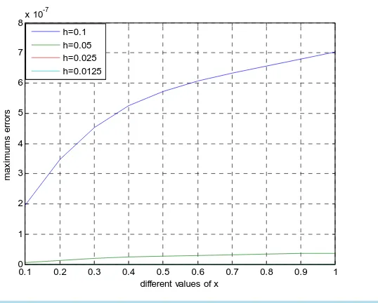
0.1 0.2 0.3 0.4 0.5 0.6 0.7 0.8 0.9 1

0 1 2 3 4 5 6 7 8x 10

-7 _{Figure 2.6:Errors for differnt step size using RK4 method}

ma

x

imu

ms

e

rr

o

rs

h=0.1 h=0.05 h=0.025 h=0.0125

Figure 14. Error for different step size using RK4 method.

solution. Also we see that the Runge Kutta approximations for same step size converge firstly to exact solution. This shows that the small step size provides the better approximation. The Runge Kutta method of order four requires four evaluations per step, so it should give more accurate results than Euler method with one-fourth the step size if it is to be superior. Finally we observe that the fourth order Runge Kutta method is converging faster than the Euler method and it is the most effective method for solving initial value problems for ordinary differ-ential equations.

6. Conclusion

In this paper, Euler method and Runge Kutta method are used for solving ordinary differential equation (ODE) in initial value problems (IVP). Finding more accurate results needs the step size smaller for all methods. From the figures we can see the accuracy of the methods for decreasing the step size h and the graph of the approxi-mate solution approaches to the graph of the exact solution. The numerical solutions obtained by the two pro-posed methods are in good agreement with exact solutions. Comparing the results of the two methods under in-vestigation, we observed that the rate of convergence of Euler’s method is O h

 

and the rate of convergence

[image:11.595.191.460.287.503.2]

(12)

From the study the Runge Kutta method was found to be generally more accurate and also the approximate solu-tion converged faster to the exact solusolu-tion when compared to the Euler method. It may be concluded that the Runge Kutta method is powerful and more efficient in finding numerical solutions of initial value problems (IVP).

References

[1] Islam, Md.A. (2015) Accuracy Analysis of Numerical solutions of Initial Value Problems (IVP) for Ordinary Differen-tial Equations (ODE). IOSR Journal of Mathematics, 11, 18-23.

[2] Islam, Md.A. (2015) Accurate Solutions of Initial Value Problems for Ordinary Differential Equations with Fourth

Order Runge Kutta Method. Journal of Mathematics Research, 7

[3] Ogunrinde, R.B., Fadugba, S.E. and Okunlola, J.T. (2012) On Some Numerical Methods for Solving Initial Value Problems in Ordinary Differential Equations. IOSR Journal of Mathematics, 1, 25-31.

[4] Shampine, L.F. and Watts, H.A. (1971) Comparing Error Estimators for Runge-Kutta Methods. Mathematics of

Com-putation, 25, 44

[5] Eaqub Ali, S.M. (2006) A Text Book of Numerical Methods with Computer Programming. Beauty Publication, Khul-na.

[6] Akanbi, M.A. (2010) Propagation of Errors in Euler Method, Scholars Research Library. Archives of Applied Science Research, 2, 457-469.

[7] Kockler, N. (1994) Numerical Method for Ordinary Systems of Initial value Problems. John Wiley and Sons, New York.

[8] Lambert, J.D. (1973) Computational Methods in Ordinary Differential Equations. Wiley, New York.

[9] Gear, C.W. (1971) Numerical Initial Value Problems in Ordinary Differential Equations. Prentice-Hall, Upper Saddle River.

[10] Hall, G. and Watt, J.M. (1976) Modern Numerical Methods for Ordinary Differential Equations. Oxford University Press, Oxford.

[11] Hossain, Md.S., Bhattacharjee, P.K. and Hossain, Md.E. (2013) Numerical Analysis. Titas Publications, Dhaka. [12] Balagurusamy, E. (2006) Numerical Methods. Tata McGraw-Hill, New Delhi.

[13] Sastry, S.S. (2000) Introductory Methods of Numerical Analysis. Prentice-Hall, India. [14] Burden, R.L. and Faires, J.D. (2002) Numerical Analysis. Bangalore, India.

[15] Gerald, C.F. and Wheatley, P.O. (2002) Applied Numerical Analysis. Pearson Education, India.