Optical approach based omnidirectional thermal visualization

Optical Approach Based Omnidirectional Thermal Visualization

Wai-Kit Wong

[email protected]

Faculty of Engineering and Technology, Multimedia University,

75450 JLN Ayer Keroh Lama, Melaka, Malaysia.

Chu-Kiong Loo

Faculty of Engineering and Technology, Multimedia University,

75450 JLN Ayer Keroh Lama, Melaka, Malaysia.

Way-Soong Lim

Faculty of Engineering and Technology, Multimedia University,

75450 JLN Ayer Keroh Lama, Melaka, Malaysia.

Abstract

In this paper, a new optical approach based on omnidirectional thermal

visualization system is proposed. It will provides observer or image processing

tool a 360 degree viewing of surrounding area using a single thermal camera. By

applying the proposed omnidirectional thermal visualization system even in poor

lighting condition, surrounding area is under proper surveillance and the

surrounding heating machineries/items can be monitored indeed. Infrared(IR)

reflected hyperbolic mirrors have been designed and custom made for the

purpose of reflecting omnidirectional scenes in infrared range for the surrounding

area to be captured on a thermal camera, thus producing omnidirectional thermal

visualization images. Five cost effective and market-common IR reflected

materials used to fabricate the designed hyperbolic mirror are studied, i.e.

stainless steel, mild steel, aluminum, brass, and chromium. Among these

materials, chromium gives the best IR reflectivity, with

. Specifically, we

introduce log-polar mapping for unwarping the captured omnidirectional thermal

image into a panoramic view, hence providing observers or image processing

tools a complete wide angle of view. Three mapping techniques are proposed in

this paper namely the point sample, mean sample and interpolation mapping

techniques. Point sample mapping technique provides the greatest interest due

to its lower complexity and moderate output image quality.

Keywords:

1. INTRODUCTION

gives the views in all direction (360 degree coverage). Such omnidirectional visualization system would be applicable in various areas, such as remote surveillance, autonomous navigation, video conferencing, panoramic photography, robotics and the other areas where large field coverage is needed.

The classical acquisition of omnidirectional images is based on the use of either mechanical or optical devices, which are discussed in details in Section 2. The mechanical solutions are based on motorized linear or array-based cameras, usually with a 360 degree rotation, scanning the visual world. The main advantage of the mechanical solution is the possibility of acquiring very high-resolution images and its major drawback is the long time requirement to mechanically scan the scene to obtain a single omnidirectional image. Hence, it cannot provide video rate real-time omnidirectional images. On the other hand, optical solutions provide lower resolution images but they are the most appropriate solutions for real-time applications. Two optical alternatives have been proposed in literature, namely the use of special purpose lens (such as fish eye lens [1]) and the use of hyperbolic optical mirrors [2]. As real-time processing and applications are intend to be investigated, only the optical approach will be pursued.

Hyperbolic optical mirror is used in this paper because it is less expensive and not complex to design as compare to fish eye lens with almost the same reflective quality. The structure for the hyperbolic optical mirror is studied and designed, as can be viewed in Section 3 in details. One goal of this research paper is to use a thermal camera to replace digital camera in order to obtain thermal/infrared (IR) visualization. Therefore, the material used to design the hyperbolic optical mirror needs to be with highest IR reflectivity. In this research paper, five different cost effective IR reflected materials, used to fabricate the designed hyperbolic mirror are studied, i.e. stainless steel, mild steel, aluminum, brass, and chromium. Among these materials, chromium gives the best outcome in IR reflectivity, with IR relative ratioεr =0.985.

The image captured from the omnidirectional thermal imaging system is not immediately understandable because of the geometric distortion introduced by the optical mirror. Hence, an unwarping process needs to be introduced in order to map the original omnidirectional thermal image into a plane that provides a complete panoramic thermal image. The advantage of such an unwarping process lays in providing the observers with a complete view of its surrounding in one image which can be refreshed at video rate. Two unwarping methods are discussed in this paper namely the pano-mapping table’s method [3] and log-polar mapping method [4]. Log-polar mapping is in favor to be selected for the proposed omnidirectional thermal visualization system because log-polar mapping does not required complicated landmark learning steps and it has lower computational complexity in calculating radial distance, comparing to pano-mapping table method. Log-polar mapping method also has higher compression capability too. Three mapping techniques for log-polar mapping are proposed in this paper namely point sample, mean and interpolation mapping techniques. Point sample mapping technique is applied in the proposed omnidirectional thermal visualization system due to its lower complexity and moderate output image quality.

The rest of the paper is organized as follows: Section 2 shows the mechanical approach versus optical approach in omnidirectional visualization and the proposed system model for our work. Section 3 presents the hyperbolic optical mirror design and discusses the materials used to construct the IR reflected hyperbolic optical mirror (or in short, omnidirectional hot mirror). Section 4 discusses two unwarping methods, namely the pano-mapping table and log-polar mapping. Three mapping techniques for log-polar mapping namely point sample, mean and interpolation mapping techniques are also discussed here. Finally, section 5 gives concluding remarks and envies some future work.

2. MECHANICAL APPROACH V.S. OPTICAL APPROACH

1.) Mechanical approach: the methods to gather images to generate an omnidirectional image.

2.) Optical approach: the methods to capture an omnidirectional image at once.

In addition, they are classified into two categories by the viewpoint of the image [5]: single viewpoint and multiple viewpoints.

For the mechanical approach, the images captured on a single viewpoint are continuous. One example is the rotating camera system [6]-[9]. In such a system, the camera rotates around the center of the lens. It generates an omnidirectional image from a single viewpoint. However, since it is necessary to rotate a video camera for a full cycle in order to obtain a single omnidirectional image, it is impossible to generate omnidirectional image at video rate. Other disadvantages of rotating camera system are that it requires the use of moving parts and precise positioning. The image captured at multiple viewpoints is relatively easy to be constructed. A single camera or more cameras are used to gather multiple images at multiple viewpoints and the images are combined into an omnidirectional image. Quick Time VR system [10] adopted such technologies and it has many market applications. However, the images generated by the system are not always continuous and consistent, and it also cannot capture the dynamic scene at video rate.

Since mechanical approach leads to many problems on discontinuity and inconsistent, optical approach is use. This approach is the most appropriate for real-time applications and it has single viewpoint. Two alternatives have been proposed, namely the use of special purpose lens (such as the fish eye lens [1]) and the use of hyperbolic optical mirrors [2]. Fish eye lens are used in place of a conventional camera lens due to the reason that they have very short focal length that enables the camera to view objects as much as in a hemisphere scene. Fish eye lens have been widely use for wide angle imaging areas as noted in [11, 12]. However, Nalwa’s works in [13] found out that it is difficult to design the fish eye lens that ensure all the incoming principal rays intersect at a single point to yield a fixed viewpoint. The acquired image, using fish eye lens, normally does not permit the distortion free perspective images constructed from the viewed scene. Hence, to capture an omnidirectional view, the design of the optimal fish eye lens must be quite complex and large, and hence expensive. Since fish eye lens are cost expensive, complex in design and providing almost the same reflective quality as hyperbolic optical mirror, hyperbolic optical approach are planned to adopt in this research.

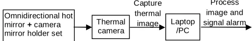
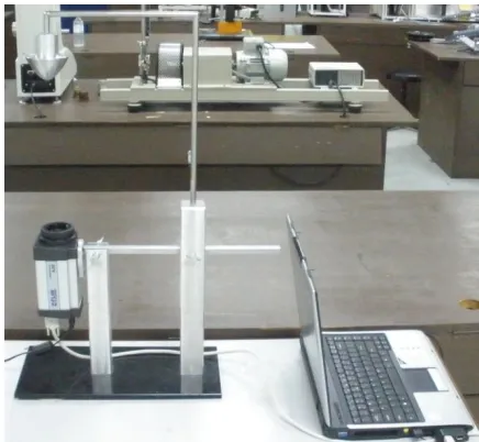
The optical approach based omnidirectional thermal visualization system model proposed in this paper is shown in Fig. 1. The system required a custom made omnidirectional hot mirror, a camera mirror holder, a fine resolution thermal camera and a laptop/PC with Matlab programming.

Fig. 1: Optical Approach Based Omnidirectional Thermal Visualization System Model

Thermal camera

Capture thermal

image Laptop /PC

Process image and signal alarm Omnidirectional hot

Fig. 2: Overall Fabricated Omnidirectional Thermal Visualization System Model

Custom made omnidirectional hot mirror will be discussed in details in Section 3. The camera mirror holder is custom designed in order to hold the camera and the omnidirectional hot mirror in a proper adjustable way. It is made with aluminum material due to its properties (light weight and acceptable tensile strength), as shown in Fig. 2.

The thermal camera used in this research is an affordable and accurate temperature model: ThermoVision A-20M manufactured by FLIR SYSTEM [14]. The thermal camera has a temperature sensitivity of 0.10 in a range from -20°C to 900°C and it can capture thermal image with fine resolution up to 320 X 240 pixels, offering more than 76,000 individual measurement points per image at a refresh rate of 50/60 Hz. The A-20M features a choice of connectivity options. For fast image and data transfer of real-time fully radiometric 16-bit images, an IEEE-1394 FireWire digital output can be chosen. For network and/or multiple camera installations, Ethernet connectivity is also available. Each A-20M can be equipped with its own unique URL allowing it to be addressed independently via its Ethernet connection and it can be linked together with router to form a network.

A laptop or PC can be used for image processor placing either on site or in a monitoring room. Matlab version 2007 or higher version is suggested because its user friendly environment (in m-file) is developed for performing log-polar mapping technique to unwrap the captured omnidirectional thermal image into panoramic form. For machine condition monitoring purposes, the software can be used to partition the panoramic thermal images easily according to each single machine to be monitored, processing them smoothly with the user-programmed monitoring algorithm and the signaling alarm whenever security threat alerts. It also can be used for trespasser detection. The overall fabricated system model is shown in Fig. 2.

3. Omnidirectional Hot Mirror

In this section, the structural design for omnidirectional hot mirror and the materials used for fabrication will be described.

3.1 Structural Design for Omnidirectional Hot Mirror

using it with a camera/imager of homogenous pixel density. Hence, it will guarantee a uniform resolution for the panoramic image after unwarping.

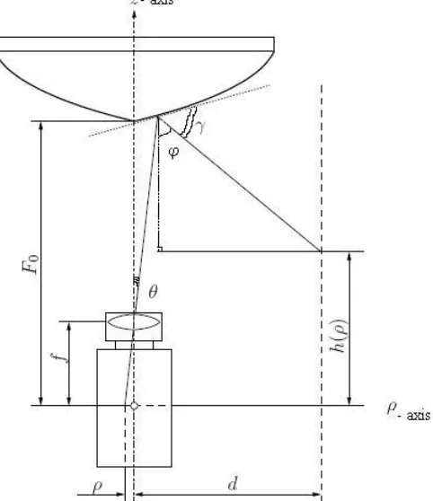
The shape of the hyperbolic omnidirectional hot mirror used in our project is design according to the derivation work done in [16,17], such that at a given distance d from the origin, the vertical dimension h is linearly mapped to the radial distance from the center of the image plane ρ as shown in Fig. 3. The relation between a world point with coordinates [d, h]T, the cross section function F(t) with t(ρ), and an image point with coordinates [ρ, 0]T is defined by the law of reflection [18], as refer to Fig. 3 and Fig. 4. According to [16], instead of deriving directly F(t), an expression for h(t) is fist sought. Referring to Fig. 3, the world point at a distance d is given by the following relation [16]:

(1)

where it carry the meaning that a ray emanating from an image point is reflected by the mirror and reaches a world point. The incident and coincident rays on the mirror [16] as shown in Fig.5 are described by their directional vectors irespectivelyc, both of norm equal to one. The law of reflection [18] imposes that the angle between incident ray and the normal to the surface is equal to the angle between the normal and the coincident ray. The normal vector n corresponds to a

Fig. 3: Mirror design structural and its related parameters.

Fig. 5: incident and coincident rays on mirror surface

function of derivatives of the cross section function F(t) at point t. Expressed in scalar product, the following condition must hold [16]:

(2)

where the components of the vectors are as follows

The law of reflection impose 2γ+θ+φ=π and therefore the slopes of the coincident ray is given by:

(3)

From (1), the term-cot(φ) can be expressed as a function of (3):

(4)

Solving (2) by substituting each respectively scalar components:

;

(5)

The condition for two unity vectors,

.

(6)

(7)

From (6),

(8)

Taking (7) divide by (8), gives

(9)

Combining (5) and (9) results in a cubic expression [16]:

(10)

Solving (10) for , get:

(11)

(12)

(11) corresponding to the slope of the transmitted ray, while (12) corresponds to the slope of the reflected ray, which is the sought one [16]. The expression for h(t) in (4) can now be written as follows:

(13)

Solving (13) for the derivative of the cross section function results in a cubic differential equation [16]:

(14)

The differential equation, which defines the convex mirror shape is consequently given by the following expression [16]:

(15)

From(15), there are three parameters influencing the mirror shape, which are the focal length

the function h(t), that corresponds to the vertical dimension of a world point. The parameter h(t) also defines the characteristic of the thermal camera. The following condition must hold [16]:

(16)

where a is the gain and b is the offset of the function in order to have a linear relationship between the coordinate of a world point and the coordinate of an image point. When substituting in (16) into (15), the image coordinate must be replaced by t. The relation between and

t results from the projection by a thermal camera as:

(17)

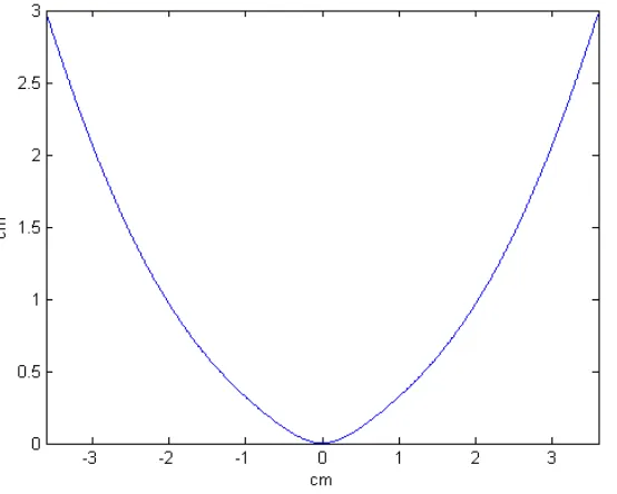
The research group of OMNIVIEWS project from Czech Technical University further developed Matlab software for designing omnidirectional optical mirror [16, 17]. From the Matlab software, practitioner can design their own hyperbolic omnidirectional hot mirror by inputting some parameters specifying the mirror dimension. The first parameter is the focal length of the camera f, in which the thermal camera in use is 12.5 mm and the distance d ( -plane) from the origin is set to 2m. The image plane height h is set to 20 cm. The radius of the mirror rim is chosen t1=3.6cm

as modified from Svoboda work in [17], with radius for fovea region 0.6cm and retina region 3.0cm. Fovea angle is set in between 0° to 45°, whereas retina angle is from 45° to 135°. The coordinates as well as the plot of the mirror shape is generated using Matlab and it is shown in Fig. 6. The coordinates as well as the mechanical drawing using Autocad was provided to precision engineering company to fabricate/custom made the hyperbolic mirror.

Fig. 6: Mirror coordinates plot in Matlab

3.2 Material for Fabricating Omnidirectional Hot Mirror

Visible light mirror’s substrate is normally glass, due to its transparency, ease of fabrication, rigidity and ability to take a smooth finish. The reflective coating is either silver (much expensive) or tin-mercury (cheaper) [20], which is applied to the back surface of the glass, so that it is protected from corrosion and accidental damage. However, this type of visible light mirror is not suitable to be applied in IR reflectivity. The reflectivity of mirror is a function of wavelength depends on both the thickness of coating and how it is applied.

Although most mirrors are designed for visible light, there are also mirrors that designed for other types of waves or wavelengths spectrum in used. The mirror that used in IR spectrum is so called “hot mirror” [21]. Hot mirror is a specialized dielectric mirror that can reflect infrared light. Normally, the materials used to build hot mirror are metals [22]. Among the metals used to fabricate hot mirror such as aluminum, silver, gold and copper based on IR reflectivity were studied by Jitra in [22]. According to the studies, the most convenient materials are silver, gold and copper because these materials have very high reflectance in IR spectral range, which is upto 90-95% of IR wavelength region [23] when they are new. If they are deposited in very thin layer, they may have high light transmittance in visible spectral range too.

However, gold and copper are very expensive materials in which they were too expensive for widespread use, as well as being prone to corrosion. They are not cost effective to be chosen for hot mirrors. And, if such hot mirrors are used on remote site, they are easily to get lost or steal by theft. Silver tends to be very soft mechanically and easily abraded, as well as susceptible to tarnishing and corrosion over time from ordinary atmospheric contaminants/conditions, such as by reacting with oxygen, chlorine, sulfur, ozone and others. Because of these reasons, silver coatings are often not used in optical mirror systems unless they are protected from the elements stated above [24]. In Jitra’s studies [22], aluminium is also not a suitable material because of its high visible reflectance.

In our research project, five types of cost effective and market-common IR reflected materials are chosen to fabricate the designed hot mirrors. They are: brass, mild steel, stainless steel, aluminum and chromium. Since fabricating mirror with whole chromium material is too expensive, it was substituted with aluminum coated with chromium. These fabricated hot mirrors are tested for reflectivity to find out the optimum one. The experimental results are shown and discussed in Section 5.1.

4. Unwarping Process

One of the important processes in optical based omnidirectional thermal visualization is the unwarping process. Unwarping process is required to map the captured omnidirectional image into a panoramic image, providing the observers and image processing tools with a complete wide angle of view for the surrounding of the area under surveillance. Many conventional unwarping methods require some information of certain omnidirectional imaging tools’ intrinsic parameters, such as lens’ focal length, coefficients of the mirror surface shape equation and the others. to perform calibration before unwarping take place [25-29]. This is not applicable in some situations where the information of such omnidirectional imaging tools’ parameters are unknown. Therefore, it is desirable to have some unwarping methods which are universal to all kinds of omnidirectional imaging tools. In this section, two such unwarping methods will be discussed, one method is the recent works of S. W. Jeng et. al. in [3] by using pano-mapping table and another one is our proposed work by the use of log-polar mapping [4].

4.1 Pano-mapping Table

The proposed work of S. W. Jeng et. al. in [3], by using pano-mapping table for unwarping omnidirectional images into panoramic view images, consists of three major stages:

as the first set of the learned data, where Oc is the image center with known world coordinates

(uo, vo) and Om is the mirror center with known world coordinates(xo, yo, zo). After learning, there

will be n sets of landmark point pairs data, each set includes the coordinates (uk, vk) of the

image point and (xk, yk, zk) of the world space point respectively, where k=0,1,…, n-1.

(ii)Table Creation Stage [3]: This stage is building a two-dimensional mapping table using the coordinates data of the landmark point pairs. The pano-mapping table is a two-dimensional array, acting as a medium for unwarping omnidirectional images, after it has been conducted. The table is shown in Table 1 below.

Θ1 Θ2 Θ3 Θ4

…

ΘM

ρ1

(u11, v11) (u21, v21) (u31, v31) (u41, v41) … (uM1, vM1)

ρ2

(u12, v12) (u22, v22) (u32, v32) (u42, v42) … (uM2, vM2)

ρ3

(u13, v13) (u23, v23) (u33, v33) (u43, v43) … (uM3, vM3)

ρ4

(u14, v14) (u24, v24) (u34, v34) (u44, v44) … (uM4, vM4)

… … … …

ρN

(u1N, v1N) (u2N, v2N) (u3N, v3N) (u4N, v4N) … (uMN, vMN)

Table 1: Example of pano-mapping table of size MxN [3].

The horizontal and vertical axes on the pano-mapping table specifies the range of the

azimuth angle Θ and the elevation angle ρ respectively of all possible incident light rays going

through the mirror center. The range 2π radians (360°) of the azimuth angles are divided equally into M-units and the range of the elevation angles are divided equally to N-units to create a table Tpm of MxN entries as shown in Table 1. Each Entry E with corresponding angle

Due to nonlinear property of the mirror surface shape, the radial-directional mapping should be specified by a nonlinear function fr, such that the radial distance r from each image pixel p with

coordinates (u, v) in I to the image center Oc at (uo, vo) may be computed by . The

pairs of all the image pixels form a polar coordinate system with the image coordinates (u, v) specified by:

In [3], the authors also name fr as the ‘radial stretching function’, and they attempt to

describe it with the following 4th degree polynomial function:

where are five coefficients to be estimated using the data of the landmark point pairs, as described in the following algorithm. A similar idea of approximation can be found in [30].

Algorithm 1. Estimation of coefficients of radial stretching [3]:

Step 1: Coordinates transformation in world space:-Transform the world coordinates (xk, yk, zk)

of each selected landmark point Pk, k=1, 2, …, n-1, with respect to origin of world

coordinate Ow into coordinates with respect to Om by subtracting from (xk, yk, zk) the

coordinates values (xo, yo, zo)=(-D, 0, H) of Om. Hereafter, (xk, yk, zk) will be denote this

coordinates transformation result.

Step 2: Elevation angle and radial distance calculation:-The coordinate’s data of each landmark point pair (Pk, pk), including the world coordinates (xk, yk, zk) and the image coordinates

(uk, vk) are use to calculate the elevation angle ρk of Pk in the world space and the radial

distance rk of pk in the image plane by the following equations:

(20)

where Dk is the distance from the landmark point Pk to the mirror center Om in the X-Y

plane of the world coordinates system, computed by .

Step 3: Calculation of coefficients of the radial stretching function:-Substitute all the data ρ0,

ρ1, …, ρn-1 and r0, r1, …, rn-1 computed in step 2 into (19) to get n simultaneous

equations:

and solve them to get the desired coefficients ( ) of the radial stretching function fr by a numerical analysis method [31].

Now the entries of the pano-mapping table Tpm can be filled with the corresponding image

coordinates using (18) and (19) with the following algorithm. Note that there are MxN entries in the table.

Algorithm 2. Filling entries of pano-mapping table [3]:

Step 1: Divide the range 2π of the azimuth angles into M intervals, and compute the i-th

azimuth angle by:

(22)

for i=0,1, …, M-1.

Step 2: Divide the range of the elevation angles into N intervals, as shown in Fig. 7, and compute the j-th elevation angle by:

(23)

for j=0,1, …, N-1.

Step 3: Fill the entry with the corresponding image coordinates (uij, vij) computed according

to (18) and (19) as follows:

where is computed by:

with being those computed by Algorithm 1.

Fig. 7: Lateral-view configuration for generating a panoramic image [3].

l

D H

Om

ρ

ρ

ρ

Panoramic

H

(iii) Image Unwarping Stage [3]: This stage is to construct a panoramic image Q using the pano-mapping table Tpm as a medium to map each pixel q in Q to an entry with coordinates

values (uij, vij) in the pano-mapping table Tpm and to assign the color value of the pixel at

coordinates (uij, vij) of image I to pixel q in Q. For the details of the generation of panoramic

image from a given input omnidirectional image I and a pano-mapping table Tpm, a

corresponding generic panoramic image Q may be generated from I, which is exactly of the same size as Tpm. The steps are as follows: First, for each entry of Tpm with azimuth angle

of and elevation angle , take out the coordinates (uij, vij) filled in , then assign the color

values of the pixel of I at coordinates (uij, vij) to the pixel of Q at coordinates (i, j). After

all entries of the table are processed, the final Q becomes a generic panoramic image corresponding to I. In the process, Q may regard as the output of the pano-mapping

described by the pano-mapping tables Tpm with I as the input, i.e. .

Pano-mapping method shows best results in unwarping omnidirectional images taken by any omnidirectional imaging tools without requirement of omnidirectional tools’ parameters. It is a universal unwarping method. However, it requires complicated landmark learning steps to define/search for different landmark points for table creation. It also has high computational complexity in which it requires up to 4th order calculation in each radial distance r as shown in Step 3 of Algorithm 1. Another demerit of such unwarping method is that it has no data compression capability. As observe from the experimental results in [3], the output panoramic image has resolution three to four folds greater than the input omnidirectional images, in which image expansion at output.

In next subsection, another universal unwarping method will be proposed, so-called the log-polar mapping method. In contrast with pano-mapping table method, log-polar mapping method does not require complicated landmark learning steps. It only needs to define one single point, which is the center of image, so-called the fovea. From the center of fovea, user can develop the fovea region and periphery region covering the whole omnidirectional image, bio-inspired the

mammalian viewing image. The computational complexity to calculate each radial distance

ρ

low, which requires cosine and sine calculation function only. Log-polar mapping method also has higher compression capability up to 4 folds.

4.2 Log-Polar Mapping

Log-polar mapping geometry is an example of foveated or space-variant image representation used in the active vision systems motivated by human visual system [32]. It is a spatially-variant image representation in which pixel separation increases linearly with distance from a central point [33]. It provides a way of concentrating computational resources on regions of interest, whilst retaining low-resolution information from a wider field of view. One advantage of this kind of sampling is data reduction. Foveal image representations like this are most useful in the context of active vision system where the densely sampled central region can be directed to pick up the most salient information. Human eyes are very roughly organized in this way.

Fig. 8: An example of log-polar mapping of a N rings retina containing 3 rings fovea. To simplify the figure, no overlapping was use. Note that periphery portion is log-polar.

The log-polar mapping can be summarized as following: Initially, the geometry of each section of the partitioned thermal image is in Cartesian form (x1,y1). Log-polar sampling is uses to sample

the Cartesian input image into log-polar sampling image. After that, the log-polar image is mapped to another Cartesian form (x2,y2) whereby in this process, the log-polar sampling image

is unwarpped into a log-polar mapping image. Since the output log-polar mapping image provides data compression and it is also in Cartesian form, subsequent image processing task will become much easier.

The centre of pixel for log-polar sampling expression is described in [4]:

(26)

(27)

The centre of pixel for log-polar mapping expression is described in [4]:

(28)

(29)

where is the distance between the given point and the center of mapping

ro is a scaling factor which will define the size of the circle at .

λ is the base of the algorithm,

(30)

is the total number of pixels per ring in log-polar geometry.

The number of rings in the fovea region is given by [4]:

To sample the Cartesian pixels (x1, y1) into log polar pixels (ρ, θ), at each center point

calculated using (1) and (2), the corresponding log-polar pixel (ρn, θn) is cover a region of

Cartesian pixels with radius:

(32)

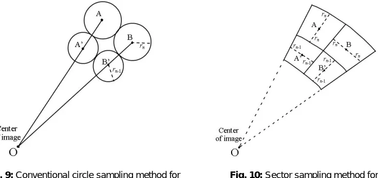
where n=0, 1, …, N-1. Fig. 9 shows the conventional circle sampling method of log-polar mapping [32, 35].

Fig. 9: Conventional circle sampling method for Fig. 10: Sector sampling method for log-polar log polar image. image.

One of the disadvantages of using circle sampling is that certain region of Cartesian pixels outside sampling circle did not cover by any log-polar pixels. Therefore, some researchers [36, 38, 39] had adopted sector sampling method as shown in Fig. 10, which could maximize the coverage of Cartesian pixels for each log-polar pixel. Log-polar pixel image will later perform mapping (unwarping) process to convert into panoramic image. There are three types of mapping techniques proposed in this paper to help generating a good quality panoramic image. They are point sample, mean and interpolation mapping technique.

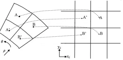
4.2.1 Point sample

Point sample is the simplest mapping techniques. During mapping process, the (ρ, θ) pixels will

map to each corresponding (x2,y2) pixels as shown in Fig. 11. The region of panoramic Cartesian

Fig. 11: Point sample mapping process 4.2.2 Mean

In mean mapping technique, the intensity value in each individual log-polar pixel equals the mean intensity value of all pixels inside the sampling sector on the original Cartesian image (x1,y1):

(33)

Fig. 12 shows the mean mapping process.

Fig.12: Mean mapping process

4.2.3 Interpolation

This method performs interpolation on point sample or mean mapping image. Interpolation is the process of determining the values of a function at the positions lying between its samples [40]. Interpolation reconstructs the information lost in the sampling process by smoothing the data samples with an interpolation function. Several interpolation methods have been developed and can be found in the literature [40- 42]. The most commonly used interpolation methods in image processing are the nearest neighbor, bi-linear and bi-cubic interpolation techniques.

(i) Nearest Neighbour Interpolation

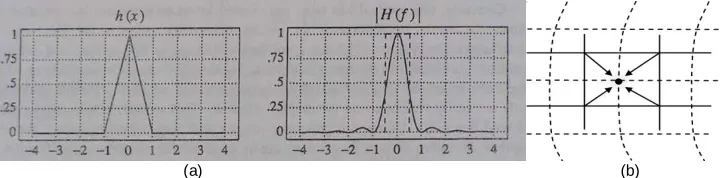
Nearest neighbor is considered the simplest interpolation method from a computational standpoint [40], where each interpolated output pixel is assigned the value of the nearest sample point in the input image. The interpolation kernel for the nearest neighbor algorithm is defined as [40]:

(34)

The frequency response of the nearest neighbor kernel is[40]:

(35)

with a sinc function [40]. Due to prominent side lobes and infinite extent, sinc function makes a poor low-pass filter. This technique achieves magnification by pixel replication, and magnification by sparse point sampling. Fig. 13b shows how the new brightness is assigned in nearest neighbor interpolation method. Dashed (- -) lines show how the inverse planar transformation map the grids of the output image into the input image (point sample or mean mapping image). Solid lines show the grid of the input image. The output pixel is assigned with the value of the pixel that the point falls within. No other pixels are considered.

(a) (b)

Fig. 13: (a) The nearest neighbor kernel and its F.T. [40] (b) Nearest neighbor interpolation

(ii) Bi-linear Interpolation

The second interpolation method discuss in this paper is bi-linear interpolation. Bi-linear interpolation explores four points neighboring the initial point, and assumes that the brightness function is bi-linear in this neighborhood. In the spatial domain, bilinear interpolation is equivalent to convolving the sampled input with the following kernel [40]:

(36)

The frequency response of the bilinear interpolation kernel is [40]:

(37)

The kernel and its Fourier transform are shown in Fig. 14a. Note that the frequency response of the bi-linear interpolation kernel is superior to the nearest neighbor interpolation since the side lobes are less prominent and the performance is improved in the stopband. A passband is moderately attenuated and this results in image smoothing. Fig 14b shows how the new brightness is assigned in bi-linear interpolation method. Dashed (- -) lines show how the inverse planar transformation map the grids of the output image into the input image (point sample or mean mapping image). Solid lines show the grid of the input image. The output pixel value is a weighted average of pixels in the nearest 2-by-2 neighborhood. Bi-linear interpolation can cause a small decrease in resolution and blurring due to its averaging nature. Bi-linear interpolation produces reasonably good results at moderate cost. But for better performance, more complicated algorithms are needed.

(a) (b)

Fig. 14: (a) The bi-linear kernel and its F.T. [40] (b) Bi-linear interpolation

(iii)Bi-cubic Interpolation

(38)

Choice for a is -1 as suggested by [43] for bicubic interpolation, (38) becomes:

(39)

The frequency response of the kernel is [40]:

(40)

The kernel and its Fourier transform are shown in Fig. 15a. Note that the frequency response of the bi-cubic interpolation preserves fine details in the image very well. Fig 15b shows how the new brightness is assigned in bi-cubic interpolation method. Dashed (- -) lines show how the inverse planar transformation map the grids of the output image into the input image (point sample or mean mapping image). Solid lines show the grid of the input image. The output pixel value is a weighted average of pixels in the nearest 4-by-4 neighborhood. Bi-cubic interpolation does not suffer from the step like boundary problem of nearest neighborhood interpolation, and copes with bilinear interpolation blurring as well.

(a) (b)

Fig. 15: (a) The bi-cubic kernel and its F.T. [40] (b) Bi-cubic interpolation

5. Experimental Results

This section will briefly illustrate the materials selected to fabricate the IR omnidirectional hot mirror, calculation on the relative permittivity of each selected materials to test for IR reflection, comparisons on the performance of the unwarping method (pano-mapping vs. log-polar mapping) and the mapping methods use in log-polar mapping (point sample, mean and interpolation).

5.1 Mirror Materials

(a) (b) (c) (d) (e)

Fig. 16: Mirror Materials (a) brass (b) mild steel (c) stainless steel (d) aluminum (e) chromium

(a) (b)

(c) (d)

Fig. 17: Case studies of machines for monitoring captured in Applied Mechanical Lab (a) Digital Color Form

(b) Thermal image, all machines are functioning in overheat condition (c)Unwarp form of a and (d) Unwarp form of b.

The panoramic form of thermal images captured on different hot mirrors are shown in Fig. 18 (a, b, c, d and e respectively). The weights and temperature readings of different hot mirrors for a selected section (machine A select as random, results will be expected same if machine B or C is choose) are recorded as shown in Table 1. The contact temperature on machine A is also measured using TES 1310 digital thermometer manufactured by TES Electrical Electronic Corp.

(a)

(c)

(d)

(e)

Fig. 18: Unwarp thermal image captured using (a) brass mirror (b) mild steel mirror (c) stainless steel mirror

(d) aluminum mirror (e) chromium mirror on the same scene.

Weight Temperature reading on Mac. A Relative reflectivity

Brass 1015g 74.2°C 0.9275

Mild steel 931g 70.8°C 0.8850

Stainless steel 940g 73.7°C 0.9213

Aluminum 325g 72.9°C 0.9113

Chromium 356g 78.8°C 0.9850

TES Thermometer NIL 80°C NIL

Table 1: weights, temperature readings and relative permittivity of different hot mirrors on a selected machine

The relative reflectivity for each hot mirror’s is calculated using the relation ratio:

(41)

where Actual temperature is the temperature measured using TES thermometer and IR reflected temperature is the temperature reflected on the hot mirror captured using thermal camera. The closest the to 1, the better the IR reflectivity of a mirror. From the experimental results shown, chromium gives the highest , with the IR reflectivity of 98.5%. This follow by brass (92.75%), stainless steel (92.13%), aluminum (91.13%) and mild steel (88.5%) respectively. Chromium is adopted in the proposed omnidirectional thermal visualization system since it provides the best IR reflectivity and its moderate weight (356g, second lightest material among the tested).

5.2 Pano-mapping vs. Log-polar Mapping

An example of omnidirectional image is taken from [3] and its pano-mapping form is shown in Fig. 19a and Fig. 19c respectively. Fig. 19b shown an unwarp panoramic form of Fig. 19a using log-polar mapping. Comparing Fig. 19b and Fig. 19c, pano-mapping method expands the panoramic image into 4 times of that original omnidirectional image, whereas log-polar mapping method has higher compression capability upto 4 folds of the original omnidirectional image. Pano-mapping method required complicated landmark learning steps whereby it is not required in log-polar mapping method. Pano-mapping method also has high computational complexity which required upto 4th order calculation in each radial distance, whereas for log-polar mapping method, the

computational to calculate each radial distance ρ is relatively low, which required 1st order cosine

(a) (b)

(c)

Fig. 19: (a) Omnidirectional image taken from [3] (b) Unwarp panoramic form of a using log-polar mapping

(c) Unwarp panoramic form of a using pano-mapping 5.3 Different Mapping Method in Log-polar Mapping

This subsection investigates different mapping methods proposed in log-polar mapping. They are point sample, mean and interpolation mapping techniques as discussed in section 4.2. Fig. 17a shows a digital image captured using the proposed chromium hot mirror as shown in Fig. 16e. As can be observed in Fig. 17a, the mirror that good in IR range does not necessary good in human visual range as well. The mapping output of Fig. 17a is shown in Fig. 20 (a to h) using different mapping techniques (point sample, mean, nearest neighbor interpolation of point sample, nearest neighbor interpolation of mean, bi-linear interpolation of point sample, bi-linear interpolation of mean, bi-cubic interpolation of point sample and bi-cubic interpolation of mean respectively). The mapping output of Fig. 17b, which is the thermal image of Fig. 17a are shown in Fig. 21 (a to h), using different mapping techniques. For interpolation techniques, the number of pixels considered affects the complexity of the computation. Therefore the bi-cubic method (weighted average of 4-by-4 neighborhood) takes longer computation times than bi-linear method (weighted average of 2-by-2 neighborhood). And, the bi-linear method takes longer times than nearest neighbor (assigned value of pixel that point nearby). However, the greater the number of pixels is considered, the more accurate the effect is; and so there is a tradeoff between processing time and quality.

(a) (b)

(c) (d)

(g) (h)

Fig. 20: Output of digital image using different mapping technique (a) point sample (b) mean (c) nearest

neighbor interpolation of point sample (d) nearest neighbor interpolation of mean (e) bi-linear interpolation of point sample (f) bi-linear interpolation of mean (g) bi-cubic interpolation of point sample (h) bi-cubic

interpolation of mean

The differences of mapping are obvious in quality for digital images but not significant in thermal images. Since interpolation and mean mapping techniques require high complexity as compare to point sample mapping technique, and all these mapping techniques provide almost the same image quality in unwarping thermal image, the less complexity technique is adopted, which is the point sample mapping technique(without interpolation).

(a) (b)

(c) (d)

(e) (f)

(g) (h)

Fig. 21: Output of thermal image using different mapping technique (a) point sample (b) mean (c) nearest

neighbor interpolation of point sample (d) nearest neighbor interpolation of mean (e) bi-linear interpolation of point sample (f) bi-linear interpolation of mean (g) bi-cubic interpolation of point sample (h) bi-cubic

interpolation of mean

6. Conclusion

providing a new platform for remote monitoring using minimum hardware. All these will be addressed in the future work.

References:

[1] J. Kumar, and M. Bauer, “Fisheye lens design and their relative performance”, Proc. SPIE, Vol. 4093, p.p. 360-369, 2000.

[2] T. Padjla and H. Roth, “Panoramic Imaging with SVAVISCA Camera- Simulations and Reality”, Research Reports of CMP, Czech Technical University in Prague, No. 16, 2000.

[3] S. W. Jeng, and W. H. Tsai, “Using pano-mapping tables for unwarping of omni-images into panoramic and perspective-view images”, IET Image Process., 1(2), p.p. 149-155, 2007.

[4] F. Berton, A brief introduction to log-polar mapping, Technical report, LIRA-Lab, University of Genova, 10 Feb 2006. [5] T. Kawanishi, K. Yamazawa, H. Iwasa, H. Takemura and N. Yokoya, “Generation of High-resolution Stereo Panoramic

Images by Omnidirectional Imaging Sensor Using Hexagonal Pyramidal Mirrors”, Proc. 14th Int. Conf. in Pattern Recognition, Vol. 1, p.p. 485-489, Aug, 1998.

[6] H. Ishiguro, M. Yamamoto, and S. Tsuji, “Omni-Directional Stereo”, IEEE Trans. Pattern Analysis and Machine Intelligence, Vol. 14, No. 2, p.p. 257-262, Feb 1992.

[7] H-C. Huang and Y. P. Hung, “Panoramic Stereo Imaging System with Automatic Disparity Warping and Seaming”, Graphical Models and Image Processing, Vol. 60, No. 3, p.p. 196-208, May 1998.

[8] S. Peleg, and M. Ben-Ezra, “Stereo Panorama with a Single Camera”, Proc. IEEE Conf. Computer Vision and Pattern Recognition, p.p. 395-401, June 1999.

[9] H. Shum, and R. Szeliski, “Stereo Reconstruction from Multi-perspective Panoramas”, Proc. Seventh Int. Conf. Computer Vision, p.p. 14-21, Sep 1999.

[10] S. E. Chen, “Quick Time VR: An Image-Based Approach to virtual Environment Navigation”, Proc. of the 22nd Annual ACM Conf. on Computer Graphics, p.p. 29-38, 1995.

[11] S. J. Oh, and E. L. Hall, “Guidance of a Mobile Robot Using an Omnidirectional Vision Navigation System”, Proc. of the Society of Photo-Optical Instrumentation Engineers, SPIE, 852, p.p. 288-300, Nov, 1987.

[12] D. P. Kuban, H. L. Martin, S. D. Zimmermann and N. Busico, “Omniview Motionless Camera Surveillance System“, United States Patent No. 5, 359, 363, Oct, 1994.

[13] V. Nalwa, “A True Omnidirecdtional Viewer”, Technical Report, Bell Laboratories, Homdel, NJ07733, USA, Feb 1996. [14] http://www.flirthermography.com

[15] J. Chahl, and M. Srinivasan, “Reflective surfaces for panoramic imaging”, Applied Optics, 36(31), p.p. 8275-85, Nov, 1997.

[16] S. Gachter, “Mirror Design for an Omnidirectional Camera with a Uniform Cylindrical Projection When Using the SVAVISCA Sensor”, Research Reports of CMP, OMNIVIEWS Project, Czech Technical University in Prague, No. 3, 2001. Redirected from: http://cmp.felk.cvut.cz/projects/omniviews/

[17] T. Svoboda, “Central Panoramic Cameras Design, Geometry, Egomotion”, PhD Thesis, Center of Machine Perception, Czech Technical University in Prague, 1999.

[18] W. C. Robertson, “Stop Faking It! Light”, National Science Teacher Association Press, 2003.

[19] J. M. Enoch, “History of Mirrors Dating Back 8000 Years”, Optometry and Vision Science, Vol. 83, Issue 10, p.p. 775-781, 2006.

[20] P. Hadsund, “The Tin-Mercury Mirror: Its Manufacturing Technique and Deterioration Processes”, Studies in Conservation, Vol. 38, No. 1, p.p. 3-16, 1993.

[21] Answer Corporation (2009) redirected from http://www.answers.com/topic/mirror

[22] J. Mohelnikova, “Materials for reflective coatings of window glass applications”, Construction and Building Materials, Elsevier, Vol. 23, Issue 5, p.p. 1993-1998, 2009.

[23] Evaporated Coating Inc., “Mirror Coatings for Plastic Optical Components” redirected from http://www.evaporatedcoatings.com/pdf/800p.pdf

[24] J. D. Wolfe, “Durable silver mirror with ultra-violet thru far infra-red reflection” Agent: James S. Tak Attorney For Applicant - Livermore, CA, US USPTO Application #: 20060141272

[25] X. H. Ying and Z. Y. Hu, “Catadioptric camera calibration using geometric invariants”, IEEE Trans. Pattern Anal. Mach. Intell., 26(10), p.p. 1260-1271, 2004.

[26] C. Geyer and K. Daniilidis, “Catadioptric camera calibration”, Proc. IEEE 7th Int. Conf. Comput. Vis., p.p. 398-404, Sep, 1999.

[27] T. Mashita, Y. Iwai and M. Yachida, “Calibration method for misaligned catadioptric camera”, IEICE Trans. Inf. Syst., E89D, (7), p.p. 1984-1993, 2006.

[28] D. Strelow, J. Mishler, D. Koes and S. Singh, “Precise omnidirectional camera calibration”, Proc. IEEE Conf. Comput. Vis. Pattern Recognit. (CVPR 2001), Kauai, HI, p.p. 689-694, Dec, 2001.

[29] D. Scaramuzza, A. Martinelli and R. Siegwart, “A flexible technique for accurate omnidirectional camera calibration and structure from motion”, Proc. Fourth IEEE Int. Conf. Comput. Vis. Syst., 2006.

[30] G. Scotti, L. Marcenaro, C. Coelho, F. Selvaggi, and C. S. Regazzoni, “Dual camera intelligent sensor for high definition 360 degrees surveillance”, IEE Proc. Vis. Image Signal Process., 152(2), p.p. 250-257, 2005.

[31] L. R. Burden and J. D. Faires, “ Numerical analysis”, Brooks cole, Belmont, C. A., 2000, 7th edition, ISBN: 0534382169.

[33] C. F. R. Weiman and G. Chaikin, “Logarithmic Spiral Grids For Image Processing And Display”, Computer Graphics and Image Processing, Vol. 11, p.p. 197-226, 1979.

[34] LIRA Lab, Document on specification, Tech. report, Espirit Project n. 31951 – SVAVISCA- available at http://www.lira.dist.unige.it.

[35] R. Wodnicki, G. W. Roberts, and M. D. Levine, “A foveated image sensor in standard CMOS technology”, Custom Integrated Circuits Conf. Santa Clara, p.p. 357-360, May 1995.

[36] F. Jurie, “A new log-polar mapping for space variant imaging: Application to face detection and tracking”, Pattern Recognition, Elsevier Science, 32:55, p.p. 865-875, 1999.

[37] V. J. Traver, “Motion estimation algorithms in log-polar images and application to monocular active tracking”, PhD thesis, Dep. Llenguatges I Sistemes Informatics, University Jaume I, Castellon (Spain), Sep, 2002.

[38] M. Bolduc and M.D. Levine, “A review of biologically-motivated space variant data reduction models for robotic vision”, Computer Vision and Image Understanding, Vol. 69, No. 2, p.p. 170-184, February 1998.

[39] C.G. Ho, R.C.D. Young and C.R. Chatwin, “Sensor geometry and sampling methods for space variant image processing”, Pattern Analysis and Application, Springer Verlag, p.p. 369-384, 2002.

[40] P. Miklos, “Image Interpolation Techniques”, 2nd Serbian-Hungarian Joint Symposium on Intelligent System (SISY 2004), p.p1-6, 2004.

Directed from: http://bmf.hu/conference/sisy2004/Poth.pdf

[41] Xin Li and Michael T. Orchard, “New Edge Directed Interpolation”, IEEE Int. Conf. on Image Processing, Vancouver,Vol.2, p.p. 311-314, Sept. 2000.

[42] Ron Kimmel, “Demosaicing: Image Reconstruction from Color CCD Samples," IEEE Trans. on Image Processing, Vol. 8, No. 9, pp. 1221-1228, September 1999.