www.ann-geophys.net/26/185/2008/ © European Geosciences Union 2008
Annales
Geophysicae
Multi-instrument observations of a large scale Pc4 pulsation
L. B. N. Clausen1, T. K. Yeoman1, R. Behlke2, and E. A. Lucek3
1Department of Physics and Astronomy, University of Leicester, Leicester LE1 7RH, UK 2Department of Physics, University of Tromsø, N-9037 Tromsø, Norway
3Department of Physics, Imperial College London, London SW7 2AZ, UK
Received: 20 June 2007 – Revised: 6 December 2007 – Accepted: 9 January 2008 – Published: 4 February 2008
Abstract. On 7 November 2005 various ground based and spaced based instruments registered five wave packets with frequencies in the Pc4 range. The most prominent of the five wave packets was observed in ground based magnetometer data spanning almost all latitudes on the dayside magneto-sphere. The propagation from the dayside into the tail is de-duced from Poynting flux calculations of Cluster data and an onset time analysis of the ground based magnetometer data. This suggests an upstream source. Backstreaming ions are identified to be the most probable source mechanism for this event. Due to the fortunate configuration of the Cluster satellites, the harmonic structure of the wave is analysed and compared with cross-phase spectra from ground data. We present evidence that the driving wave resonantly interacted with geomagnetic field lines. The data suggests that reso-nant driving occurred at stations where the driving frequency was harmonically related to the local fundamental frequency, creating FLR-like signatures.
Keywords. Magnetospheric physics (MHD waves and in-stabilities; Solar wind-magnetosphere interactions) – Space plasma physics (Waves and instabilities)
1 Introduction
In the dayside magnetosphere, ultra-low frequency (ULF) pulsations with spectral power in the Pc4 frequency range are abundant. The Pc4 interval ranges from 7 to 22 mHz (pe-riods between 45 and 150 s) and the “Pc” reflects the fact that these pulsations tend to be continuous. They also occur less abundantly on the nightside.
Nightside Pc4 pulsations seem to be linked to substantial substorm activity, usually occurring two to four hours after-wards (e.g. Nos´e, 1998). Particle data suggests that these
pul-Correspondence to: L. Clausen
sations are driven via a wave-particle interaction by freshly injected hot ions. Since most events occur during overall quiet geomagnetic times, a small convective electric field might also play a role. Through similar wave-particle in-teractions ions injected during substorms also drive Pc4 pul-sations with high azimuthal wave numbers predominantly in the morning sector (Baddeley et al., 2002).
On the dayside, Pc4 pulsations are thought to originate from either Kelvin-Helmholtz instabilities on the magne-topause (Greenstadt et al., 1979) or wave-particle instabili-ties in the Earth’s upstream region (Troitskaya et al., 1971; Le et al., 2000). An analysis of the occurrence region and propagation of the wave packets later in this paper will point towards the second mechanism, hence we can ignore the first mechanism in the context of this study.
When the orientation of the interplanetary magnetic field (IMF) is roughly (anti-)parallel to the normal vector of the bow shock, ions can be reflected at the boundary and travel upstream. Here they resonantly interact with naturally occur-ring waves, amplifying them (Barnes, 1970; Sentman et al., 1981). Since upstream the bow shock the solar wind is supersonic, these waves are then convected with the solar wind flow into the magnetosphere. Numerical hybrid models have been used to show that these fast/magnetosonic waves can then pass through the turbulent bow shock and magne-tosheath into the dayside magnetosphere, leaving their spec-trum mainly unchanged (Krauss-Varban, 1994).
Having reached the magnetosphere, compressional Pc3-4 waves are detected by space based instruments (e.g. Chi and Russell, 1998) and on the ground by magnetometers. On the ground they appear usually as large scale waves with low azimuthal wave numbers (Odera et al., 1991). Several em-pirical relations have been derived to predict the upstream generated frequency from IMF conditions (e.g. Le and Rus-sell, 1996).
Continuous pulsations at latitudes above 60◦are generally observed at lower frequencies between 2 and 7 mHz (periods between 150 and 600 s) and these are termed Pc5 pulsations (e.g. Samson et al., 1992). Due to the lengths of the field lines at these latitudes the Pc5 range is favoured and Pc4 would only be expected if the density along the field lines was significantly lower than normal.
High latitude Pc5 pulsations often have distinctive char-acteristics and they have are known as field line resonances (FLR). Dungey proposed that they are standing Alfv´en waves on geomagnetic field lines, a concept that has been confirmed by a number of studies (e.g. Walker et al., 1979). Since Chen and Hasegawa (1974) and Southwood (1974) have shown that energy from compressional wave modes can couple to Alfv´enic modes, it is commonly accepted that compressional waves generated at either the Earth’s bow shock or through solar wind buffeting can couple to FLRs where the frequen-cies match. Since the requirements are only met by a small fraction of field lines, FLRs tend to be latitudinally localized. In this paper we discuss a highly coherent Pc4 pulsation with amnumber around unity. It is a global phenomenon, occurring at both low and high latitudes, over 12 h of mag-netic local time (MLT). We explore the possibility of it be-ing a FLR and investigate its source usbe-ing ground and space based magnetometer data.
2 Observations
On 7 November 2005 between 13:10 and 14:10 UT over two dozen ground based magnetometers around the world registered five wave packets in the upper end of the Pc4 range. During this time, the magnetic foot prints of Cluster 3 and 4 of the four Cluster satellites (Escoubet et al., 2001) were, according to the Tsyganenko 96 (T96) model (Tsyga-nenko, 1995), conjunct with magnetometers belonging to the CARISMA array located in Canada. The CARISMA array spans magnetic latitudes from 60◦to 80◦and magnetic lon-gitudes from 270◦to 330◦. For the time discussed here, this translated to MLTs between 04:00 and 09:00, i.e. on the dawn flank of the magnetosphere. At the same time and nearly symmetric to the morning side stations, magnetometers be-longing to the SAMNET and IMAGE arrays on the evening side between 14:00 and 17:00 MLT registered the same os-cillations. These stations span magnetic latitudes from 50◦ to 75◦at magnetic longitudes between 70◦and 120◦. 2.1 Ground based magnetometers
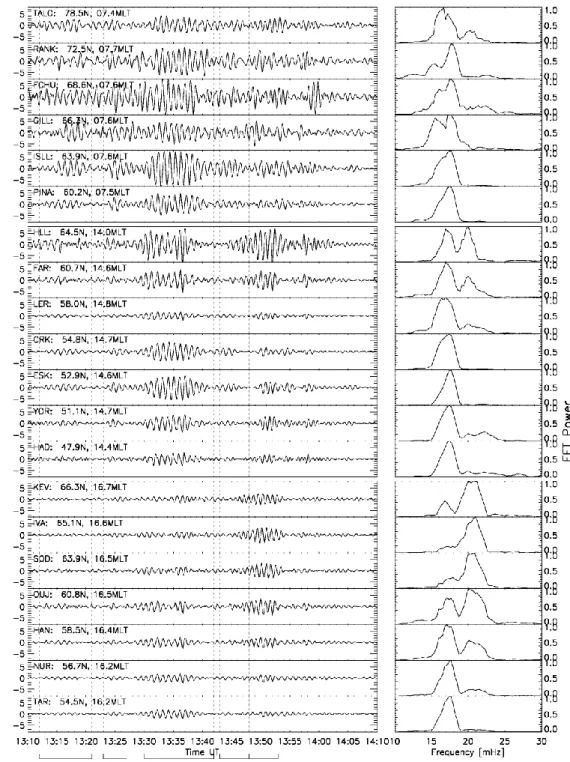
Figure 1 shows the X (North-South) component of the mag-netic field as measured by magnetometers along three lati-tude profiles at different MLTs in the left panels. The data have been bandpass filtered between 20 and 80 s. The mag-netic latitude of each station and its MLT is given next to its abbreviation in the top left hand corner of each panel. The
right hand side panels show the Fourier spectrum of the fil-tered time series, each individually normalized. The spectra have been smoothed using a five points wide boxcar average to eliminate spikes.
As indicated in Fig. 1 by vertical dashed lines, five sepa-rate ULF wave packets can be identified at all stations. The first between 13:12 and 13:21 UT, the second between 13:23 and 13:27 UT, the third between 13:30 and 13:42 UT, the fourth between 13:43 and 13:48 UT and the fifth between 13:48 and 13:53 UT. The focus of this study lies on the wave packet which occurred between 13:30 and 13:42 UT. It was the most prominent of the five, already well defined in unfil-tered data.
Basic Fourier analysis of the interval between 13:10 and 14:10 UT shows that the frequency of the first four pul-sations was 17.2±1.0 mHz whereas the last oscillated at 20.2±1.0 mHz (see right panels in Fig. 1). The power at 20.2 mHz dominates the power spectra of the northern IM-AGE stations SOD, IVA, KEV, whereas in all other spectra the 17.2 mHz peak is dominant. The frequency of each wave packet was constant over all latitudes. Although not imme-diately apparent from Fig. 1, cross-correlation techniques re-veal that all five packets can in fact be seen in the data of all stations. The bandwidth of the filter in Fig. 1 was chosen such that any power at double the dominant frequency, i.e. at 34 mHz, is not filtered. There was, however, no signature present at this frequency.
The top six panels of Fig. 1 show the data of a line of magnetometers belonging to the CARISMA array in Canada spanning about 20◦ in magnetic latitude, located around 07:00 MLT. The amplitude distribution of the third wave packet over latitude has two maxima, at ISLL and FCHU. Both phase and onset time vary with latitude, however the frequency does not. There is a distinct 180◦phase shift be-tween the time series of GILL and FCHU but only a very small shift across the latitude of ISLL. Therefore the ampli-tude and phase profile over FCHU are indicative for the fact that the observed pulsation is at these stations is a FLR.
When studied in detail the pulsation between 13:30 and 13:42 UT consisted of two overlapping yet separate wave packets. SAMNET and IMAGE data (bottom panels in Fig. 1) show this more clearly than data from CARISMA stations. The further north the station, the further apart the two wave packets appeared. Since the pulsation occurred si-multaneously at all stations, this indicates that it was a spatial feature rather than a temporal one.
Fig. 1. Bandpass filtered (20 to 80 s) ground based magnetometer data from three latitudinal profiles using CARISMA, SAMNET and
IMAGE stations on the left. Five pulsation events are marked by vertical dashed lines. The panels on the right show the normalized smoothed Fourier spectra.
considering stations up to LER (58◦N), latitude profiles of phase and power show FLR-like behaviour.
At higher latitudes, the oscillation consisted of two pack-ets, as seen in data from CARISMA stations. However, since SAMNET stations reach to lower latitudes, the merge was completed below 54◦(CRK) such that the oscillation then seemed to consist of only one wave packet.
Table 1. Phase in degree at 17.2 mHz for different stations along
longitudinal profiles determined by Fourier analysis.
Dawn Dusk
Name Long. Phase Name Long. Phase DAWS‡ 273 −59
FSIM‡ 294 −37 DOB? 090 −40 FSMI‡ 306 −24 HAN? 104 −47 RABB‡ 318 −04 MEK? 108 −53
Diff. 45 55 18 −13
m −1.2 0.7
‡CARISMA stations
?IMAGE stations
latitudes into two at higher latitudes was again observed. To determine the azimuthal wave numberm of the ob-served pulsation, phase shifts at stations along longitudinal profiles both on the dusk and dawn side have been analysed. The phase of the 17.2 mHz component was obtained from Fourier analysis of the unfiltered signal. A summary is given in Table 1. Themnumber is then obtained by dividing the observed phase shift by the longitudinal separation. By con-vention the eastward direction is associated with positivem
numbers.
With increasing longitude the phase increases on the morning side, corresponding to a negative m number and westward propagation. On the evening side, the phase de-creases with increasing longitude resulting in a positivem
number, equivalent to eastward propagation. This corre-sponds in both cases to a propagation of the wave in an anti-sunward direction. The absolute value is in both cases around one, confirming that this wave was a large-scale phe-nomenon.
Although it is not shown, it is worth noting that pulsa-tion signatures identical to those described above were ob-served on the dayside by magnetometers located on Green-land, South America and Antarctica. These wave packets were clearly a global magnetospheric phenomenon with the exact same frequency at all stations. From these additional sources only the Antarctic stations yielded enough power for analysis, however due to the low power construction of these magnetometers, the time stamp associated with each mea-surement is uncertain by up to two minutes, thus rendering these data useless for timing analysis.
[image:4.595.64.272.98.231.2]Weak but coherent signals of the pulsation described here were also recorded at stations located on the nightside. Data from Japanese magnetometers at magnetic latitudes between 20◦and 40◦and 23:00 MLT show pulsations at 17.2 mHz with amplitudes around 0.2 nT. Magnetometers in Alaska (60◦magnetic latitude, 03:00 MLT) recorded the pulsation with an amplitude of 1 nT.
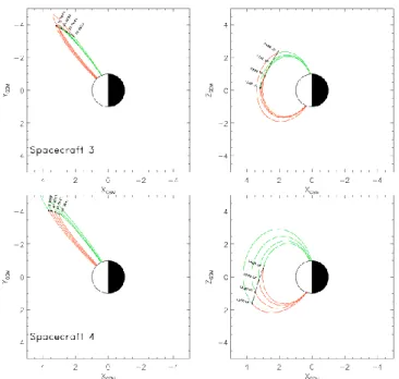
Fig. 2. Cluster 3 (top two panels) and 4 (bottom two panels) orbit.
Also shown is the T96 model geomagnetic field with input parame-terspdyn=2.0 nPa,Dst=0.0,By,IMF=0.0 nT,Bz,IMF=0.0 nT.
2.2 Space based observations
The formation of the Cluster satellites during the event was rather like pearls on a string. Cluster 2 was leading, followed by Cluster 1, 3 and 4, each separated by about 2 Re. Their or-bit took them from the southern hemisphere through perigee at about 5 Reover the northern hemisphere to apogee into the tail. Due to this orbit configuration, Cluster 3 and 4 sampled the magnetic and electric field variations along essentially the same bundle of field lines (see Fig. 2). At the time of the wave event Cluster 1 and 2 had already passed the inner magnetosphere and were on open field lines connected to the northern polar cap. Hence only Cluster 3 and 4 data can be used in this study.
The magnetic field was measured by the FGM (Balogh et al., 2001) instrument on board the Cluster satellites. It is available in GSE coordinates at spin resolution (4 s). The electric field data used in this study was gathered by the EFW (Gustafsson et al., 1997) instrument. They were provided by the Cluster Active Archive and consist of two components in the GSE X-Y plane, also at spin resolution. The third com-ponent was calculated under the frozen flux assumption, i.e. E+v×B=0. It then follows that the electric and magnetic field ought to be orthogonal, i.e.E·B=0 which yields
Ez= −(ExBx+EyBy)/Bz. (1)
The results of the above calculation have to be treated very carefully whenever Bz is close to zero. However,
of the order 200 nT, thus conveniently having avoided this problem.
After theEzcomponent has been calculated from the raw
magnetic and electric field data following Eq. (1), all compo-nents have been bandpass filtered to allow periods between 20 and 80 s and then transformed into a local dipole aligned coordinate system (LDC).
In this orthogonal system the background magnetic field is assumed to be purely dipolar. This assumptions is justi-fied by the geocentric distance of the satellites of only 5 Re. One axis points along the background dipole magnetic field, such that positive values denote variations parallel to the lo-cal dipole field. The second axis points azimuthally, parallel to the X-Y GSM plane, positive eastward. The third axis completes the right hand system by pointing positive radi-ally inwards. Thus, for magnetic field data the field aligned time series will contain the compressional component, the azimuthal direction will contain transverse toroidal oscilla-tions and the radial component will contain the transverse poloidal oscillations.
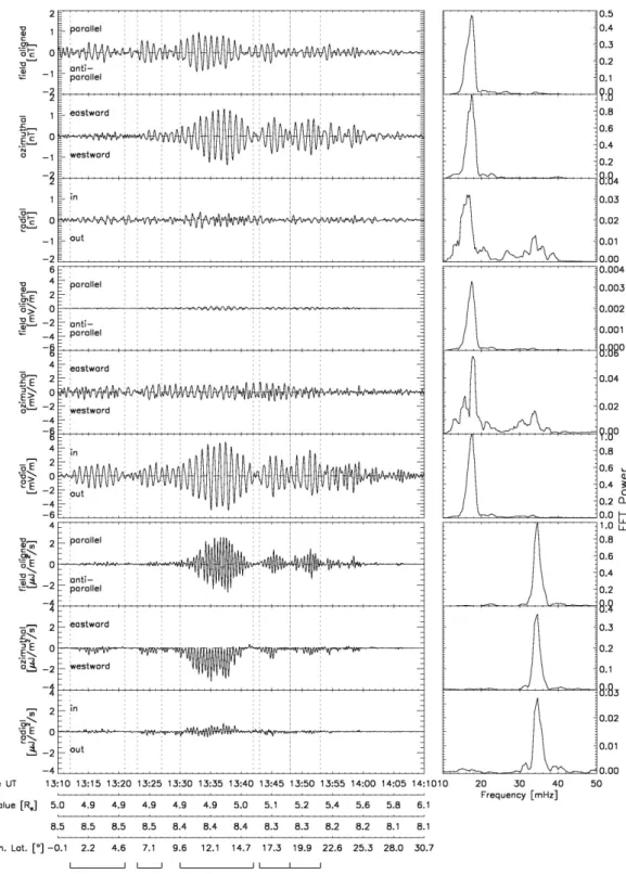
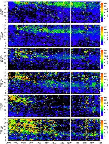
The right panels in Fig. 3 show the Fourier spectra for the filtered time series. The spectral powers have been smoothed using a five point wide boxcar average to eliminate spikes. Then the spectra were normalized by the maximum value of each component for each quantity individually. Please note that the range of the y axis is not the same for all spectra.
The left panels show time series of the magnetic and elec-tric field and the oscillatory Poynting flux. All quantities are plotted versus time, L-value, MLT and magnetic latitude of the spacecraft. The dipole tilt angle respective to the Z-GSM axis during the event was about−9◦.
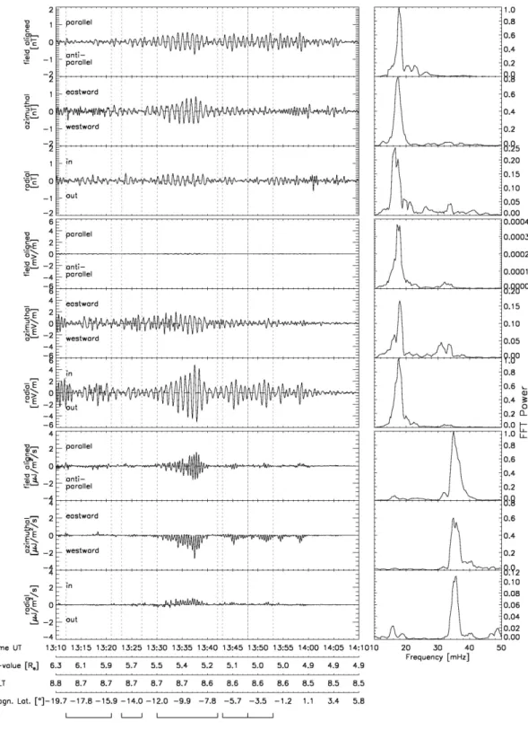
The top three left panels in Fig. 3 and Fig. 4 show the fil-tered components of the magnetic field for Cluster 3 and 4 in the LDC, respectively. All five wave packets are clearly vis-ible in the data and the polarization of the wave is revealed. The variation at 17.2 and 20.2 mHz was confined to the field aligned and azimuthal direction, showing that the wave con-sisted of a superposition of a transverse toroidal and a com-pressional mode. This is true for data from both Cluster 3 and 4.
The Fourier spectra show that the compressional and poloidal component of Cluster 3 magnetic field as well as the toroidal electric field contained a weak signal at double the main frequency, i.e. at 34 mHz. The same is true for the Cluster 4 data.
The envelopes of the main pulsation seen by the FGM on board Cluster 3 and 4 in the field aligned components show under close inspection two maxima, whereas the azimuthal components show only one.
The amplitude of the pulsation as seen by Cluster 3 was about twice that seen by Cluster 4. Whereas the signal in the field aligned direction had no phase shift between the two spacecraft the oscillation in the azimuthal direction was 180◦ out of phase.
The electric field shown in panels four to six in Fig. 3 and 4 also shows a clear polarization in the local dipole coordinate system. The bulk of the power was concentrated in the ra-dial direction with all five wave packets clearly visible. The azimuthal component shows an elevated level of what seems to be incoherent noise. There was a coherent oscillation at 17.2 mHz in the field aligned direction. The ratio of radial to field aligned amplitude was about ten at Cluster 3 and four at Cluster 4, making the field aligned component more signifi-cant at Cluster 4. The signals from both satellites in the radial direction were in phase, as were the field aligned. A consid-erable difference in the packet’s envelope was observed.
From the three components of the electric fieldeand the magnetic fieldbthe three components of the Poynting vector shave been calculated via
s= 1
µ0
(e×b). (2)
Sinceswas calculated from the filtered components it repre-sents the Poynting flux of the wave field only.
Due to the polarization ofeandbin the LDC the Poynting vector was polarized as well, having comparable amplitudes in the field aligned and azimuthal component (see Fig. 3 and Fig. 4 bottom three panels). The period of the oscillation was, as expected, double that ofeandb. The field aligned com-ponent ofsfor Cluster 3 showed a slight asymmetry around the zero line, indicating more flux parallel to the background magnetic field than anti-parallel. Since Cluster 3 was lo-cated about 12◦above the magnetic equator, this indicates that some of the wave’s energy was lost in the northern po-lar ionosphere. The same is true for observations at Cluster 4 position, however here the energy was lost in the negative field aligned direction into the southern hemisphere, in accor-dance with the satellites position at−10◦magnetic latitude.
The azimuthal flux at both satellites was, considering their position in the magnetosphere, purely tailward, i.e. west-ward, negative azimuthally. The asymmetries in both the field aligned/azimuthal flux is a direct and sole result of phase shift between the azimuthal/field aligned magnetic and radial electric field components at both satellites.
The small signals in the field aligned direction of the elec-tric field results in some flux in a radially inward direction, more so at Cluster 4.
3 Discussion
3.1 Wave motion and origin
Fig. 3. Summary of field data in local dipole coordinates from Cluster 3. The top three panels show the magnetic field, followed by the
electric field and the oscillatory Poynting flux. The right hand side panels show the respective smoothed Fourier spectra.
Cluster tetrahedron gives us the unique opportunity to study the structure of the wave along a bundle of field lines and thus explore the wave’s harmonic mode.
As discussed earlier, the magnetic field and Poynting flux data suggests that the wave was composed of two modes,
Fig. 4. Summary of field data from Cluster 4, same layout as Fig. 3.
was also highly asymmetric. Virtually all flux was directed tailward. This leads to the assumption of an anti-sunward travelling compressional wave from which energy was lo-cally converted into the Alfv´enic mode. The pulsations seen by the ground based magnetometers are then due to these Alfv´enic oscillations.
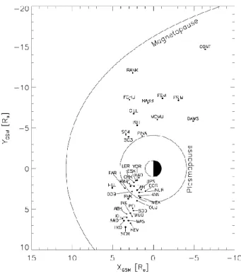
Fig. 5. Equatorial crossing points of field lines adjacent to ground
magnetometer stations in GSM coordinates. The magnetopause po-sition was calculated according to Shue et al. (1997). The plasma-pause is shown following Larsen et al. (2007).
The geographic positions of each magnetometer belonging to the CARISMA, IMAGE and SAMNET chain have been traced along the adjacent field line into the equatorial plane of the GSM coordinate system (see Fig. 5), thus finding each station’s cross-point. The tracing utilised the T96 model with input parameters derived from measurements of the GEO-TAIL satellite (pdyn=1.5 nPa, Dst=−15.0, By,IMF=−1.5 nT,Bz,IMF=−0.5 nT). Due to the finite step size of the T96 model, the Z values of the equatorial positions were not zero, however they were less than 0.2 Refor all stations.
To determine the onset time of at each station, the filtered time series between 13:30 and 13:42 UT of each station of the three chains have been cross-correlated with the time se-ries of one reference station. HAD from the SAMNET chain was chosen to be the reference since it is the station in which time series the pulsation occurred first.
The sample interval of IMAGE stations is ten seconds as opposed to one second for SAMNET stations, therefore be-fore cross-correlation the reference data have been downsam-pled by calculating the average over ten seconds. The same procedure was applied before cross-correlating the reference data with the four second sampled Cluster magnetic field measurements. Finally the onset time was then determined by extracting the lag of the maximum cross-correlation.
[image:8.595.52.281.62.322.2]Tamao (1964) investigated the propagation of a MHD wave from a point source through a cold uniform plasma.
Fig. 6. MHD wave propagation inside the Earth’s magnetosphere
from a source Q to an observerP1,P2,P3,P4on the ground. The
path shown is that identified by Tamao (1964) as the least attenuated one.
He then applied his findings qualitatively to a MHD wave propagating through the magnetosphere to an observer on the ground.
The source Q emits compressional waves in all directions, as indicated by the dotted concentric lines in Fig. 6. These waves travel with the local Alfv´en speed as the plasma is as-sumed to be cold, and they are attenuated asr−1,rbeing the distance from the source. Along its path the fast mode con-stantly converts to the Alfv´en mode, which then travels along the magnetic field line without further attenuation toP1,P2,
P3,P4, the observer on the ground. Hence most power is transported to the ground by a path which minimised the length the wave travels in fast mode. This path is depicted in Fig. 6 as a straight arrow in blue from the source to the field line connected toP1,P2,P3,P4, followed by the red arrow indicating the Alfv´en mode travelling along the mag-netic field line. This method was successfully used by Chi et al. (2001) to explain arrival times of preliminary reverse impulses.
Additional to the lag time due to different paths of the wave to the observer on the ground, the phase shifts result-ing from an internal resonance structure of the pulsation will influence the observed onset times. Whereas the wave prop-agation along different paths will constitute the bulk of the lag time, the internal resonance structure of the pulsation can only change the lag times by±30 s, i.e.±one half period.
2001)
ρ(r)= (
ρps rppr
3
, r≤rpp
ρms rmp
r
3
, r > rpp
(3)
For each station in Fig. 5 the travel time along a straight line from the source to the cross-point was calculated us-ing Eq. (3) to model the density profile. The travel time of the Alfv´enic mode along the magnetic field line as predicted by the T96 model was than added. Finally, the minimum travel time of all stations was subtracted from all travel times such that these relative times can be compared to the relative times determined by the afore mentioned cross-correlation technique.
Optimal values for the mass densities were found by sys-tematically varying these parameters until the best agree-ment between observation and model was reached. ρps
was varied between 25 amu/cm3and 300 amu/cm3in steps of 25 amu/cm3. The magnetospheric density was varied between 0.25 amu/cm3 and 2.0 amu/cm3 in 0.25 amu/cm3 steps. For each pair of density values model travel times were computed. The standard deviation of the differences between model and observational time lags of all stations has been used as a quantifier for the goodness of fit of the input density values. The densities producing the smallest deviation were then chosen as the optimal input parameters for our model. These values wereρms=0.75 amu/cm3andρps=50 amu/cm3
which achieved a minimal standard deviation of 7.8 s. A plasmaspheric density ofρps=50 amu/cm3seems rather
low, however note that changing this value to a more sensi-ble value of 150 amu/cm3 increases the standard deviation marginally from 7.8 to 8.4 s. On the other hand changing the magnetospheric density from 0.75 to 1.5 amu/cm3increases the standard deviation to over 12 s.
As mentioned earlier, the observational lag times of some stations might have been affected by additional time shifts due to local resonance effects. However the spread of the station’s positions over large parts of the dayside of the mag-netosphere both in MLT and L-shell (compare Fig. 5) means that only few of the stations will have been affected by such additional shifts. Hence this intuitive measure for the good-ness of the model is suitable for this situation.
The geocentric distance of the plasmapause was derived from a recent model by Larsen et al. (2007). They found that the following parameters strongly correlate with the plasmapause position: the IMF Z-GSM componentBz, IMF
clock angleθ=arccos(Bz/
q B2
y+Bz2)and a merging proxy
φ=V Bsin(θ/2)2, whereV is the solar wind speed andBis the IMF magnitude. The delay in the plasmapause response to the changing parameters was found to be 180 min forBz,
175 min forθand 240 min forφ. According to Larsen et al. (2007) the plasmapause positionLpp can then be calculated
[image:9.595.308.550.57.302.2]via
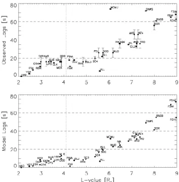
Fig. 7. Observed lag times (top panel) and relative predicted lag
times (bottom panel). The dotted vertical line indicates the mod-elled plasmapause stand-off distance. The error bars in the top panel are due to the different sampling frequencies of the different mag-netometers.
Lpp[Re] =0.050Bz,180+0.108θ175 (4) −1.110×10⁻⁴φ240+4.23,
which in this case yieldsrpp=4.1 Re. Please note that this model does not account for the MLT dependence ofLpp.
For our calculations the magnetopause position was as-sumed to lie atrmp=10 Re. To find the location of the
up-stream source its position was varied using the same scheme as for the mass densities. For 80 points along a line paral-lel to the Y-GSM axis at ZGSM=0 Re and XGSM=10 Re be-tween−4 Re≤YGSM≤4 Rethe model lag time and the stan-dard deviation of the difference between the lag times were calculated. It was found that the best agreement, i.e. the lowest standard deviation, between observation and model is achieved when assuming the source to lie at (10, 0, 0) Re. This position is consistent with what will be inferred about the wave’s origin later in this section.
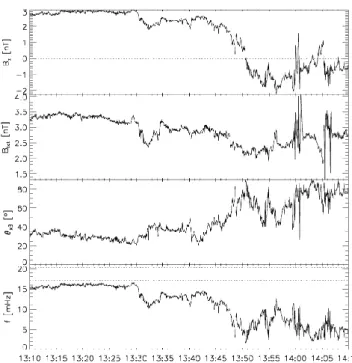
Fig. 8. Magnetic field data from GEOTAIL. The cone angleθxB
and the predicted upstream generated frequencyfpred are shown
in the two bottom panels. The two horizontal dotted lines in the bottom panel show the observed frequencies.
are well reproduced by the model. Please bear in mind that the time resolution for the IMAGE magnetometers is 10 s such that the observed lags can only be determined to that accuracy.
All the above observations suggest an upstream source, hence the solar wind data has been analysed for possible triggers of the observed wave. Possible triggers for ULF waves in the magnetospheric cavity include increased shear flow at the magnetopause, generating waves through Kelvin-Helmholtz-Instabilities or solar wind buffeting due to oscil-lations or sudden changes in the solar wind dynamic pres-sure. The first option is unlikely, seeing that the maximum shear flow is achieved at the flanks of the magnetosphere. However, the onset time analysis suggests propagation of the wave essentially along the X GSM axis as opposed to origi-nating from one of the flanks. The second option is ruled out since no oscillations in the solar wind dynamic pressure can be observed during the interval of interest.
Another wave generation mechanism is through instabili-ties between the solar wind plasma and ions backstreaming from the Earth’s bow shock. Backstreaming ions are pre-dominantly observed at a quasi-parallel shock, i.e. when the shock normal and the magnetic field vector are close to being (anti-)parallel. A generally used condition is that the angle between the two vectors is smaller than 30◦. To our knowl-edge, two similar empirical models have been developed to estimate the frequency generated by this mechanism, one by
Takahashi et al. (1984) and one by Le and Russell (1996). Both models are parametrized by the IMF strengthBtotin nT and the cone angleθxB as defined by
cos(θxB)= |Bx|/Btot. (5)
Here we use the more recent relation found by Le and Rus-sell (1996) which is based on linear theory. It states that the predicted frequencyfpred[mHz]is dependent onBtotandθxB as
fpred[mHz] = 0.72+4.67 cos(θxB)Btot. (6) During the event, the GEOTAIL satellite was located in-side the solar wind close to the Earth’s bow shock on the evening side. From its magnetic field dataθxB was
calcu-lated and the frequency of the upstream generated waves at the subsolar point has been estimated using the Eq. (6) (see Fig. 8). The predicted frequency matches reasonably well with the frequency observed, however Eq. (6) predicts slightly lower frequencies than those observed.
3.2 Harmonic structure
The cross-phase technique was employed (Kurchashov et al., 1987; Waters et al., 1991) to estimate the natural frequency of field lines. We can then investigate whether and how the observed oscillation was related to a normal mode of the con-sidered field lines.
Under two assumptions one can estimate the natural (fun-damental) frequency of a field line by calculating the cross-phase spectrum of two adjacent stations at similar longi-tudes but different latilongi-tudes. Firstly it is assumed that quasi-random variations at the natural frequency of the field line are always present in the data. Secondly, the natural frequency of the poleward station is, mainly due to the longer field line, slightly lower than that of the equatorward station. The nat-ural frequency of the field line located half way between the two stations is then that frequency, at which the cross-phase spectrum reaches its maximum. It has been shown (e.g. Wa-ters et al., 1991) that this technique is reasonably robust in de-termining the natural frequency, even at low signal strengths. The results for some exemplary SAMNET stations are shown in Fig. 9. The decreasing frequency with increas-ing latitude is nicely visible, as well as an expected varia-tion of the fundamental frequency with local time (Waters et al., 1995). This technique yields clearer results for data from the evening flank. However, due to the symmetry of the CARISMA station and SAMNET station locations, conclu-sions drawn from the latter may be applicable to the morning sector (compare Fig. 5).
The natural frequency decreases with increasing L-value, with a steeper gradient inside the plasmasphere than inside the magnetosphere. The position of the plasmapause can be identified as the position of a “bump” in the curve, as indi-cated by an arrow in Fig. 10. Its location coincides with the result derived from Eq. (4) as marked by the dotted vertical line. The results presented here are very similar to those pre-sented in Fig. 3 of Menk et al. (2004). Least-square fitting a straight line to the data points in the two regimes as indicated by the solid lines in Fig. 10 yields two functional dependen-cies of the fundamental frequencyffundon L-valueL:
log10ffund(L)= (
2.17−0.33L, L.4Re
1.20−0.04L, L&4Re (7) During the fitting process the two points comprising the bump in Fig. 10 have been excluded. Using the above for-mula, an individual fundamental frequency for each station in Fig. 5 can be calculated.
It was already remarked that ground based magnetometer data show maximal amplitudes at two different latitudes. In an attempt to explain this amplitude distribution, the natural frequency of each station in Fig. 5 was plotted against the spectral power of each station’s time series at 17.2 mHz.
The idea is that the amplitude of the pulsation and thus the spectral power at 17.2 mHz of the ground based data was higher at latitudes, where the driving pulsation was harmon-ically related to the fundamental frequency because the driv-ing wave could then have resonantly interacted with the local field line.
Panel a of Fig. 11 shows the spectral power at 17.2 mHz over the fundamental frequency. The colours indicate the sta-tion’s chain, blue for SAMNET stations, orange for IMAGE and green for CARISMA. The station abbreviations are given above or below their respective circle. The vertical bold dashed line marks the frequency of the driving pulsation, i.e. 17.2 mHz. The second vertical dashed line at 6.5 mHz indi-cates the fundamental frequency of the field line whose sec-ond harmonic frequency matches the driving frequency.
The harmonic relationship for geomagnetic field line eigenfrequencies was studied for a dipole magnetic field by Schulz (1996). He found the frequency ratios at L=6 for the toroidal eigenmodes to bef2/f1=2.63 (compare Table 1 in Schulz, 1996). For different L-values the ratio varies by about 0.25. In Fig. 11 this variation has been indicated by a gray band.
The lower panels of Fig. 11 show latitude profiles of the phase of selected stations determined by FFT analysis. Panel b shows a latitude profile of CARISMA stations and panel c of SAMNET stations. The same stations as plotted in the lower panels are connected by lines in panel a.
[image:11.595.308.550.62.382.2]The reader is reminded that the fundamental frequency of a field line is inversely proportional to the latitude of its foot point, i.e. the higher the latitude, the lower the fundamental frequency. Hence, Fig. 11 can also be looked at as a latitude
Fig. 9. Cross-phase spectra of stations belonging to the SAMNET
array.
Fig. 10. Fundamental frequency over L-value. CARISMA stations
are coloured green, SAMNET stations are blue and IMAGE stations are orange. The dotted vertical line indicates the position of the plasmapause predicted by Eq. (4).
profile of spectral power. For an ideal FLR such a profile shows a peak in power at the latitude of the resonant field line, accompanied by a 180◦phase shift across that latitude.
[image:11.595.307.549.431.574.2]Fig. 11. (a) Fundamental frequency against the spectral power at
17.2 mHz. CARISMA stations are coloured green, SAMNET sta-tions are blue and IMAGE stasta-tions are orange. (b) Latitude profile of the FFT phase of selected CARISMA stations; these are con-nected by straight lines in panel (a). (c) Latitude profile of the FFT phase of selected SAMNET stations; these are connected by straight lines in panel (a).
wave and the local field lines took place. This is due to the overall small signal strength at these stations combined with an unfortunate position of the fundamental frequencies be-tween the two frequencies marked in Fig. 11.
The spectral powers of a latitude profile of stations be-longing to the SAMNET array (HAD, YOR, ESK, CRK and LER) have been connected by straight lines in Fig. 11. The accompanying Fourier phases have been plotted in panel c. Both plots provide strong evidence that across this latitude (∼54◦ magnetic latitude), where the driving and local fun-damental frequency matched, resonant interaction took place and a FLR was generated.
The fundamental frequency at BOR was, according to Fig. 11, also close to that of the driving wave. Hence an en-hancement in power could be expected. However, the power at BOR is low due to the station’s position at 17:00 MLT where wave power is usually low. Conversely, power at HLL is high although its fundamental frequency is not close to any of the frequencies where resonant interaction is expected. Hence the amplitude distribution of the SAMNET data can only partly be explained by resonant interaction of the driv-ing wave with a local field line.
A second latitude profile at higher latitudes on the dawn side consisting of CARISMA stations has also been marked in Fig. 11. It consists of the stations PINA, ISLL, GILL, FCHU, RANK. The corresponding Fourier phases are shown
in panel b. Ignoring the power value at ISLL for a moment, again a clear signature of a FLR emerges. This indicates that the driving wave generated a FLR on the dawn side at a latitude where the second harmonic frequency of the local fundamental matched the driving frequency.
The above discussion shows that our idea of resonant in-teraction can only explain parts of the amplitude distribution of the Fourier powers with latitude. The high power values at ISLL and HLL remain puzzling because their fundamen-tal frequency was not harmonically related to the driving fre-quency.
As can be seen in Fig. 2, the two Cluster satellites were located along the same bundle of field lines during the entire event. This, together with the global, simultaneous appear-ance of the wave in ground based magnetic data, strongly in-dicates that the observed wave packets were a temporal rather than a spatial feature. The separation of the two spacecraft was 2 Reon the same field line, therefore phase information from the magnetic and electric field data can be used to learn more about the spatial structure of the wave along the field line.
The cross-phase method was used to determine the rela-tive phase shift of the Fourier component at 17.2 mHz and its evolution during the event for the field-aligned and az-imuthal magnetic component (not shown) between the two spacecraft. The phase difference of the field-aligned compo-nent was constant at about 0◦, whereas the phase shift in the azimuthal component was constant at 180◦.
Because of the finite L-shell difference between Cluster 3 and 4, a measurable difference in resonance frequency at the two positions can be expected. Hence the relative phase between the signals of the two spacecraft would change with time if at their position a resonance would be observed. Since this is not the case, this confirms the observation that the Cluster satellites do not observe the signal of a resonating field line but that of an almost monochromatic driver.
Since the compressional parts of the magnetic field were in phase, the following considerations are only valid for the Alfv´enic mode. The phase shift of the azimuthal magnetic components between the two spacecraft was 180◦, whereas the radial electric components were in phase. Numeri-cally solving the decoupled first-order wave equation along a dipole magnetic field line as derived in Sinha and Rajaram (1997) yields solutions for the magnetic and electric field. The following observations are qualitative and are only con-cerned with the node structure of the oscillation.
The density profile along the field line was assumed to be
ρ=ρ0 r0
r n
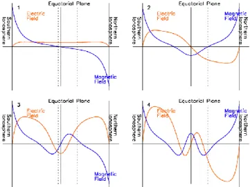
[image:12.595.46.288.60.294.2]Fig. 12. Numerical solution of the wave equation on a dipolar field
line. The first four harmonics are shown. Superimposed are the scaled positions of the Cluster 3 (right of the equatorial plane) and 4 (left) spacecraft.
aroundn=1. For calculations this value was chosen and it is worth noting that variations of the density index did not significantly change the positions of the nodes.
The result of a numerical integration using the standard fourth-order Runge-Kutta method is shown in Fig.. 12. Note that the delineation shows, for the sake of clarity, the two quantities at times of maximum amplitude. Superimposed are the positions of the Cluster spacecraft as dashed lines. Since the dipole field line in this sketch is represented by a straight line, the positions of the spacecraft have been scaled accordingly.
The numerical solution in Fig. 12 is based on the assump-tion that conductivities in both the northern and southern ionosphere are identical. This assumption does not hold for the position of the field lines adjacent to the Cluster satellites during the time of the event. The ionosphere at the southern foot point of the involved field lines was sun lit, whereas it was not at the northern end. Hence the ionospheric conduc-tivities are expected to be lower at the northern than at the southern foot point. However, Streltsov and Lotko (1997) investigated the influence of finite ionospheric conductiv-ity on the structure of dispersive, nonradiative FLRs for the first four odd harmonics. Their results are based on a lin-ear, magnetically incompressible, reduced, two-fluid MHD model which includes effects of finite electron inertia (at low altitude) and finite electron pressure (at high altitude). They found that assuming different conductivities for the north-ern (6P=2 mho) and southern (6P=∞mho) ionospheres
[image:13.595.46.287.63.243.2]do not significantly change the positions of the nodes. The first and fourth harmonics seem possible solutions to explain the observed spatial phase shifts of the wave field, i.e. 0◦between the two radial electric and 180◦between the two azimuthal magnetic fields. Sch¨afer et al. (2007) found
Fig. 13. Resulting wave structure when a 17.2 mHz wave is fed
into the Runge-Kutta algorithm. The vertical dashed lines again show the scaled positions of the Cluster spacecraft 3 (right of the equatorial plane) and 4 (left).
that the fundamental eigenfrequency of a toroidal standing wave on a dipole field line atL=5 Reunder similar magne-tospheric conditions is about 13 mHz. Similar values around 10 mHz can be extracted by eye from the cross-phase spectra of data from the morning side ground based magnetometers. Hence it is more likely that the observed wave at 17.2 mHz at the Cluster position has a node structure related to the funda-mental or the second harmonic rather than one related to the fourth harmonic.
When feeding the Runge-Kutta algorithm with a 17.2 mHz wave and assuming that the electric field had a node only on one end of the field line, the picture as delineated in Fig. 13 emerges. It has the same format as Fig. 12. Under the as-sumption that the electric field had a node in the northern hemisphere, the observed phase shifts in the Cluster data can be reproduced.
The astute reader will notice that the southern end of the field line connects to the sun-lit hemisphere. There the con-ductivities were probably higher than at the dark northern foot point. Hence the node in the electric field is more likely to have been in the southern end as opposed to the northern as delineated in Fig. 12. However, the observed phase shifts in the Cluster data can only be reproduced when assuming the node in the electric field to have been at the northern foot point. It is possible that auroral precipitation changed the local ionospheric conductivities at the foot print of the field lines connected to the satellites such that the above scenario becomes plausible.
On 7 November 2005 five wave packets in the Pc4 fre-quency range have been observed in ground based magne-tometer data from stations spanning virtually all latitudes and all MLTs. The most prominent of the wave packets had a frequency of 17.2 mHz and an azimuthal wave numbermof about 1. The frequency was constant at all latitudes.
by backstreaming ions at the Earth’s bow shock. The com-pressional part of this wave then propagated through the bow shock and the magnetosheath into the magnetosphere. There its energy partially converted into Alfv´enic modes which were observed as a global phenomenon by ground instru-ments. Space based instruments registered both modes.
Due to the unique spatial arrangement of two Cluster spacecraft the harmonic structure of the wave packet along the same bundle of field lines has been studied. A simple comparison between the phase shifts of the azimuthal mag-netic and radial electric field between the two spacecraft and numerical solutions of the wave field suggests that at an L-value of 5 Reon the dawn flank the observed pulsation had a node structure similar to the fundamental of the adjacent field line. However uncertainties in the numerical solution exist that could effect the node structure and hence its inter-pretation.
Using the cross-phase technique, fundamental frequencies of field lines adjacent to ground based magnetometers have been calculated and compared with that of the observed pul-sation and the Cluster observations. At latitudes comparable with that of the Cluster foot print these data suggest that the pulsation was oscillating at a frequency between the local fundamental and second harmonic frequency. This observa-tion is supported by the observed phase shift at the Cluster satellites and numerical simulations.
On the dusk side the incident wave generated a FLR at a latitude where the local fundamental frequency matched the driving frequency. On the dawn side indications for a FLR are found across the latitude where the driving frequency matched the second harmonic of the local fundamental.
Some of the features of the discussed event remain puz-zling. The high amplitudes observed on the ground at HLL and ISLL cannot be explained by resonant interaction of lo-cal field lines and the driving wave (see Fig. 11). The split-ting of the wave packet as observed on the ground could be due to different damping rates at different latitudes (see Fig. 1). Lower damping at lower latitudes could be responsi-ble for the merging of two wave packets into what appears to be one. And lastly the signal at double the main frequency in the spacecraft data (see Fig. 3 and 4) could be connected to mechanisms described in Takahashi and McPherron (1982), Higuchi et al. (1986) and Mann et al. (1999).
Acknowledgements. L. Clausen acknowledges funding from the
European Commission under the Marie Curie Host Fellowship for Early Stage Research Training SPARTAN, Contract No MEST-CT-2004-007512, University of Leicester, UK.
The authors would like to thank the following people and institu-tions for providing data and maintaining instruments: I. R. Mann at the University of Alberta and the CARISMA team, CARISMA is operated by the University of Alberta, funded by the Cana-dian Space Agency; A. Viljanen at the Finnish Meteorological In-stitute and the IMAGE team; F. Honary at Lancaster University and the SAMNET team, SAMNET is a PPARC National Facil-ity operated by Lancaster UniversFacil-ity; A. Balogh at Imperial
Col-lege and the Cluster/FGM team; M. Andre at the Swedish Insti-tute of Space Physics and the Cluster/EFW team; the Cluster Active Archive team; T. Nagai at the Tokyo Institute of Technology and the GEOTAIL/MGF team. GEOTAIL/MGF data was provided through DARTS at the Institute of Space and Astronautical Science (ISAS) in Japan.
The authors would also like to thank C. Waters of the University of Newcastle, Australia, for providing code for calculating cross-phase spectra.
Topical Editor I. A. Daglis thanks K. Takahashi and M. Vellante for their help in evaluating this paper.
References
Baddeley, L. J., Yeoman, T. K., Wright, D. M., Davies, J. A., Trat-tner, K. J., and Roeder, J. L.: Morning sector drift-bounce res-onance driven ULF waves observed in artificially-induced HF radar backscatter, Ann. Geophys., 20, 1487–1498, 2002. Balogh, A., Carr, C. M., Acu˜na, M. H., Dunlop, M. W., Beek, T. J.,
Brown, P., Fornac¸on, K.-H., Georgescu, E., Glassmeier, K. H., Harris, J., Musmann, G., Oddy, T., and Schwingenschuh, K.: The Cluster Magnetic Field Investigation: Overview of In-Flight Performance and Initial Results, Ann. Geophys., 19, 1207–1217, 2001.
Barnes, A.: A theory of generation of bow-shock-associated hydro-magnetic waves in the upstream interplanetary medium, Cosmic Electrodyn., 1, 90–+, 1970.
Chen, L. and Hasegawa, A.: A theory of long-period magnetic pul-sations, 1. Steady state excitation of field line resonance, J. Geo-phys. Res., 79, 1024–1032, 1974.
Chi, P. J. and Russell, C. T.: Phase skipping and Poynting flux of continuous pulsations, J. Geophys. Res., 103, 29 479–29 492, doi:10.1029/98JA02101, 1998.
Chi, P. J., Russell, C. T., Raeder, J., Zesta, E., Yumoto, K., Kawano, H., Kitamura, K., Petrinec, S. M., Angelopoulos, V., Le, G., and Moldwin, M. B.: Propagation of the preliminary reverse impulse of sudden commencements to low latitudes, J. Geophys. Res., 106, 18 857–18 864, doi:10.1029/2001JA900071, 2001. Denton, R. E., Goldstein, J., Menietti, J. D., and Young, S. L.:
Magnetospheric electron density model inferred from Polar plasma wave data, J. Geophys. Res., 107, 25–1, doi:10.1029/ 2001JA009136, 2002.
Escoubet, C. P., Fehringer, M., and Goldstein, M.: The Cluster Mis-sion, Ann. Geophys., 19, 1197–1200, 2001.
Greenstadt, E. W., Olson, J. V., Loewen, P. D., Singer, H. J., and Russell, C. T.: Correlation of PC 3, 4, and 5 activity with solar wind speed, J. Geophys. Res., 84, 6694–6696, 1979.
Gustafsson, G., Bostrom, R., Holback, B., Holmgren, G., Lundgren, A., Stasiewicz, K., Ahlen, L., Mozer, F. S., Pankow, D., Harvey, P., Berg, P., Ulrich, R., Pedersen, A., Schmidt, R., Butler, A., Fransen, A. W. C., Klinge, D., Thomsen, M., Falthammar, C.-G., Lindqvist, P.-A., Christenson, S., Holtet, J., Lybekk, B., Sten, T. A., Tanskanen, P., Lappalainen, K., and Wygant, J.: The Elec-tric Field and Wave Experiment for the Cluster Mission, Space Sci. Rev., 79, 137–156, 1997.
Krauss-Varban, D.: Bow Shock and Magnetosheath Simulations: Wave Transport and Kinetic Properties, in: Solar Wind Sources of Magnetospheric Ultra-Low-Frequency Waves, edited by: En-gebretson, M. J., Takahashi, K., and Scholer, M., 121–134, 1994. Kurchashov, I. P., Nikomarov, I. S., Pilipenko, V. A., and Best, A.: Field line resonance effects in local meridional structure of mid-latitude geomagnetic pulsations, Ann. Geophys., 5, 147–154, 1987.
Larsen, B. A., Klumpar, D. M., and Gurgiolo, C.: Correlation be-tween plasmapause position and solar wind parameters, J. At-mos. Terr. Phys., 69, 334–340, doi:10.1016/j.jastp.2006.06.017, 2007.
Le, G. and Russell, C. T.: Solar wind control of upstream wave frequency, J. Geophys. Res., 101, 2571–2576, doi:10.1029/ 95JA03151, 1996.
Le, G., Chi, P. J., Goedecke, W., Russell, C. T., Szabo, A., Petrinec, S. M., Angelopoulos, V., Reeves, G. D., and Chun, F. K.: Mag-netosphere on May 11, 1999, the Day the Solar Wind Almost Disappeared, II Magnetic Pulsations in Space and on the Ground, Geophys. Res. Lett., 27, 2165–+, 2000.
Mann, I. R., Chisham, G., and Wanliss, J. A.: Frequency-doubled density perturbations driven by ULF pulsations, J. Geophys. Res., 104, 4559–4566, doi:10.1029/1998JA900136, 1999. Menk, F. W., Mann, I. R., Smith, A. J., Waters, C. L., Clilverd,
M. A., and Milling, D. K.: Monitoring the plasmapause using geomagnetic field line resonances, J. Geophys. Res., 109, 4216– +, doi:10.1029/2003JA010097, 2004.
Nos´e, M.: ULF pulsations observed by the ETS-VI satellite: Sub-storm associated azimuthal Pc4 pulsations on the nightside, Earth Planets Space, 50, 63–80, 1998.
Odera, T. J., van Swol, D., Russell, C. T., and Green, C. A.: PC 3,4 magnetic pulsations observed simultaneously in the magne-tosphere and at multiple ground stations, Geophys. Res. Lett., 18, 1671–1674, 1991.
Samson, J. C. and Rostoker, G.: Latitude-dependent characteristics of high-latitude Pc 4 and Pc 5 micropulsations, J. Geophys. Res., 77, 6133–6144, 1972.
Samson, J. C., Harrold, B. G., Ruohoniemi, J. M., Greenwald, R. A., and Walker, A. D. M.: Field line resonances associated with MHD waveguides in the magnetosphere, Geophys. Res. Lett., 19, 441–444, 1992.
Sch¨afer, S., Glassmeier, K. H., Eriksson, P. T. I., Pierrard, V., Fornac¸on, K. H., and Blomberg, L. G.: Spatial and temporal characteristics of poloidal waves in the terrestrial plasmasphere: a CLUSTER case study, Ann. Geophys., 25, 1011–1024, 2007.
Schulz, M.: Eigenfrequencies of geomagnetic field lines and im-plications for plasma-density modeling, J. Geophys. Res., 101, 17 385–17 398, doi:10.1029/95JA03727, 1996.
Sentman, D. D., Edmiston, J. P., and Frank, L. A.: Instabilities of low frequency, parallel propagating electromagnetic waves in the earth’s foreshock region, J. Geophys. Res., 86, 7487–7497, 1981. Shue, J.-H., Chao, J. K., Fu, H. C., Russell, C. T., Song, P., Khurana, K. K., and Singer, H. J.: A new functional form to study the solar wind control of the magnetopause size and shape, J. Geophys. Res., 102, 9497–9512, doi:10.1029/97JA00196, 1997.
Sinha, A. K. and Rajaram, R.: An analytic approach to toroidal eigen mode, J. Geophys. Res., 102, 17 649–17 657, doi:10.1029/ 97JA01039, 1997.
Southwood, D. J.: Some features of field line resonances in the magnetosphere, Planet. Space Sci., 22, 483–491, 1974.
Streltsov, A. and Lotko, W.: Influence of the finite ionospheric con-ductivity on dispersive, nonradiative field line resonances, Ann. Geophys., 15, 625–633, 1997.
Takahashi, K. and McPherron, R. L.: Harmonic structure of Pc 3-4 pulsations, J. Geophys. Res., 87, 1504–1516, 1982.
Takahashi, K., McPherron, R. L., and Terasawa, T.: Dependence of the spectrum of Pc 3-4 pulsations on the interplanetary magnetic field, J. Geophys. Res., 89, 2770–2780, 1984.
Tamao, T.: The Structure of Three-dimensional Hydromagnetic Waves in a Uniform Cold Plasma, J. Geomagn. Geoelectr., 16, 89–114, 1964.
Troitskaya, V. A., Plyasova-Bakunina, T. A., and Gul’elmi, A. V.: Relationship between Pc 2-4 pulsations and the interplanetary field, Dokl. Akad. Nauk. SSSR, 197, 1313, 1971.
Tsyganenko, N. A.: Modeling the Earth’s magnetospheric magnetic field confined within a realistic magnetopause, J. Geophys. Res., 100, 5599–5612, 1995.
Walker, A. D. M., Greenwald, R. A., Stuart, W. F., and Green, C. A.: STARE auroral radar observations of Pc 5 geomagnetic pulsa-tions, J. Geophys. Res., 84, 3373–3388, 1979.
Waters, C. L., Menk, F. W., and Fraser, B. J.: The resonance struc-ture of low latitude Pc3 geomagnetic pulsations, Geophys. Res. Lett., 18, 2293–2296, 1991.