Improved error control techniques for data transmission

(1)

Improved Error Control Techniques for Data

Transmission

Steven Robert Marple

Submitted for the degree of

Doctor of Philosophy.

University of Lancaster.

(2)

(3)

List of Figures

2.1 Array code. . . 13

2.2 Encoder for (2;1;3) convolutional code. . . 24

2.3 Concatenated coding example. . . 26

2.4 Trellis for RM(8;4;4) with definitions. . . 30

2.5 Binary symmetric channel model. . . 33

2.6 Binary symmetric erasure channel model. . . 35

4.1 Component Syndrome Trellises for RS(7;5;3). . . 83

4.2 Syndrome trellis for RS(7;5;3). . . 85

4.3 A trellis isomorphic to the RS(7;5;3) syndrome trellis. . . 86

4.4 Component Coset trellises for RS(7;3;5). . . 92

4.5 Coset trellis For RS(7;3;5). . . 93

4.6 A discrete symmetric channel model. . . 96

4.7 Soft-decision Viterbi decoding example. . . 97

4.8 Flowchart of the Viterbi decoding algorithm. . . 99

4.9 Trellis for RM(8;4;4). . . 104

5.1 Signalling values with PDFs for Eb=N0 = 3 dB superimposed. . . 121

(10)

LIST OF FIGURES viii

5.2 Scaled LL metrics for coherently-demodulated BPSK. . . 124

5.3 Variation of LL metrics for a BPSK channel . . . 125

5.4 Example trellis with metric differences for traceback SOVA. . . 127

5.5 Flowchart of the soft output Viterbi decoding algorithm. . . 130

5.6 Soft-decision Viterbi decoding example with soft outputs. . . 132

5.7 Cascade decoding algorithm for product code. . . 138

5.8 Alternating row/column decoding example. . . 145

6.1 Calculating the state metric. . . 155

6.2 Algebraic decoding performance for RS(7;5;3). . . 162

6.3 Algebraic decoding complexity for RS(7;5;3). . . 170

6.4 Two-stage decoding of RS(7;3;5), with HD choice of subtrellis. . . . 175

6.5 Two-stage decoding of RS(7;3;5), with SD choice of subtrellis. . . . 176

6.6 Two-stage decoding of RS(7;5;3), with HD choice of subtrellis. . . . 177

6.7 Two-stage decoding of RS(7;5;3), with SD choice of subtrellis. . . . 178

6.8 Subset of RS(7;5;3) trellis for u2 =0;u3 =0. . . 179

6.9 Subset of RS(7;5;3) trellis for u2 =1;u3 =2. . . 180

6.10 Subsets of RS(7;5;3) trellis for u2 =f0;1g, u3 =f0;2g. . . 181

6.11 One section of the (2;1;7) convolutional code trellis. . . 186

(11)

LIST OF FIGURES ix

6.16 Comparison of alternating row-column decoding algorithms. . . 199

6.17 Iterative alternating row-column decoding. . . 201

(12)

List of Tables

3.1 Solution to Example 3.1. . . 48

3.2 Solution to Example 3.2. . . 50

3.3 Galois field elements for GF(16). . . 53

3.4 Syndrome values. . . 54

3.5 Solution of the Key Equation using Euclid’s algorithm. . . 56

3.6 Solution of the Key Equation using BM algorithm. . . 62

3.7 High-speed step-by-step decoding of RS(15;9;7). . . 72

4.1 Channel metrics for the Viterbi decoding example. . . 95

4.2 Symbol predictors for Two-stage decoding of RS(7;3;5). . . 110

4.3 Symbol predictor results. . . 112

4.4 Soft GF arithmetic for GF(4). . . 113

5.1 Transition probabilities and LL metrics for a BPSK channel. . . 123

5.2 Sample codewords of the non-systematic RS(7;5;3) trellis. . . 136

5.3 Sample codewords of the systematic RS(7;5;3) trellis. . . 136

6.1 Relative complexity of algebraic operations (for a DSP32C). . . 152

(13)

LIST OF TABLES xi

6.2 Comparison of VA and SOVA decoding complexity for RS(7;3;5). . . 160

6.3 Comparison of VA and SOVA decoding complexity for RS(7;5;3). . . 160

6.4 Complexity for decoding RS(7;3;5). . . 164

6.8 Complexity versus subtrellises decoded for TSD of RS(7;3;5). . . 173

6.9 Complexity versus subtrellises decoded for TSD of RS(7;5;3). . . 174

6.10 Specifications of simulated Meteosat II system. . . 183

6.11 Additional coding gain achieved through use of SOVA. . . 188

6.12 Complexity for VA decoding of the convolutional (2;1;7) code. . . . 193

6.13 Complexity for SOVA decoding of the convolutional (2;1;7) code. . . 193

6.14 Comparison of decoding complexity for the Meteosat II concatenated coding scheme. . . 193

6.15 Binary to GF(8) mapping for LL metrics. . . 194

(14)

Acknowledgements

I would like to take this opportunity to thank my supervisor, Professor B. Honary,

for his guidance, support and encouragement. Without this help I could not have

completed this work.

I would also like to thank my colleagues, both past and present, in the

Communi-cations Research Centre, Department of CommuniCommuni-cations, Lancaster University.

Finally, I would like to thank my parents and Judith for their support.

(15)

Declaration

This Thesis and the work described in it are my own, except where stated otherwise.

The work was carried out at the University of Lancaster between January 1994 and

December 1999. No part of this Thesis has been submitted for the award of a higher

degree, either at the University of Lancaster or elsewhere. Some parts of this Thesis

have appeared in publications, which are listed below and in the References.

B. Honary, G. Markarian, and S. Marple. Trellis decoding of block codes:

Practical approach. In ICCT ’96, volume 1, pages 525–527, Beijing,

China, May 1996.

Relevant Thesis sections: 4.1.2, 4.1.4, 4.2.5, 4.3, 6.1.2, 6.2, and 6.4.

B. Honary, G. Markarian, and S. R. Marple. Trellis decoding of the

Reed-Solomon codes: Practical approach. In 3rd International Symposium on

Communication Theory and Applications, pages 12–16, Ambleside, UK,

July 1995.

Relevant Thesis sections: 4.1.2, 4.1.4, 4.2.5, 4.3, and 6.4.

(16)

DECLARATION xiv

B. Honary, G. Markarian, and S. R. Marple. Two-stage trellis decoding of

RS codes based on the Shannon product. In Proceedings of the 1996

In-ternational Symposium on Information Theory and Its Applications, pages

282–285, Victoria, BC, Canada, September 1996.

Relevant Thesis sections: 4.1.2, 4.1.4, 4.2.5, 4.3, 6.1.2, 6.2 and 6.4.

B. Honary, G. Markarian, and S. R. Marple. Trellis decoding of the

Reed-Solomon codes: A practical approach. In B. Honary, M. Darnell,

and P. G. Farrell, editors, Communications Coding and Signal Processing,

Communications Systems Techniques and Applications Series, pages 133–

147. John Wiley & Sons, New York, London, Sydney, 1997. ISBN

0 86380 221 4.

Relevant Thesis sections: 4.1.2, 4.1.4, 4.2.5, 4.3, 6.1.2, 6.2, and 6.4.

B. Honary and S. R. Marple. Investigation of sequence segment keying

(SSK) and its application in CDMA systems. In ITEC 96, Leeds, UK,

April 1996.

(17)

Symbols and Abbreviations

ARC alternating row-column [decoding]

AWGN additive white Gaussian noise

B branch profile

BCH Bose-Chaudhuri-Hocquenghem

BCH(n;k;d) BCH code with given parameters

BCJR Bahl-Cocke-Jelinek-Raviv [trellis]

BER bit error rate

BM Berlekamp-Massey [decoding]

BPSK binary phase shift keying

BSC binary symmetric channel

C code

CCSDS Consultative Committee on Space Data Systems

CPU central processing unit

d minimum distance

DMC discrete memoryless channel

e error vector

(18)

SYMBOLS AND ABBREVIATIONS xvi

e error symbol

e(x) error polynomial

Eb bit energy

ESA European Space Agency

FSK frequency shift keying

FSR feedback shift-register

G generator matrix

g(x) generator polynomial

GAC generalised array code

GF Galois field

H parity-check matrix

HD hard decision

HDMLD hard decision maximum-likelihood decoding

HSSBS high-speed step-by-step [decoding]

K constraint length of a convolutional code

k number of information symbols in block code

L label profile

LL log likelihood

MAP maximum a posteriori

MDS maximum distance separable

ML maximum-likelihood

N state profile

(19)

SYMBOLS AND ABBREVIATIONS xvii

N0 noise spectral density

NASA National Aeronautics and Space Administration

Pb probability of bit error

PDF probability density function

PM probability of block error

Ps probability of symbol error

q alphabet size used by a code

QPSK quaternary phase-shift keying

r received codeword vector

r received codeword symbol

r degree of generator polynomial

r(x) received codeword polynomial

RM Reed-Muller

RM(n;k;d) Reed-Muller code with given parameters

RS Reed-Solomon

RS(n;k;d) Reed-Solomon code with given parameters

S syndrome vector

S(x) syndrome polynomial

SD soft decision

SDMLD soft decision maximum-likelihood decoding

SNR signal to noise ratio

SOVA soft-output Viterbi algorithm

(20)

SYMBOLS AND ABBREVIATIONS xviii

t maximum number of correctable errors

TSD two-stage decoding

u dataword vector

u dataword symbol

u(x) dataword polynomial

v codeword vector

v codeword symbol

v(x) codeword polynomial

VA Viterbi algorithm

primitive element of Galois field

discrepancy

complexity

(x) error-locator polynomial

(x) correction polynomial for(x)

number of correctable errors

(x) error-evaluator polynomial

(21)

Abstract

Error control coding is frequently used to minimise the errors which occur naturally in

the transmission and storage of digital data. Many methods for decoding such codes

already exist. The choice falls mainly into two areas: hard-decision algebraic

decod-ing, a computationally-efficient method, and soft-decision combinatorial decoddecod-ing,

which although more complex offers better error-correction.

The work presented in this Thesis is intended to provide practical decoding

algo-rithms which can be implemented in real systems.

Soft-decision maximum-likelihood decoding of Reed-Solomon codes can be

ob-tained by using the Viterbi algorithm over a suitable trellis. Two-stage decoding of

Reed-Solomon codes is presented. It is an algorithm by which near-optimum

perfor-mance may be achieved with a complexity lower than the Viterbi algorithm.

The soft-output Viterbi algorithm (SOVA) has been investigated as a means of

providing soft-decision information for subsequent decoders. Considerations of how

to apply SOVA to multi-level codes are given. The use of SOVA in a satellite downlink

channel is discussed. The results of a computer simulation, which showed a 1:8 dB

improvement in coding gain for only a 20% increase in decoding complexity, are

(22)

ABSTRACT xx

presented.

SOVA was also used to improve the decoding performance when applied to an RS

product code. Several different decoding methods were evaluated, including cascade

decoding, and a method where the row and columns were decoded alternately.

A complexity measurement was developed which allows accurate comparisons of

decoding complexity for trellis-based and algebraic decoders. With this technique the

decoding complexity of all the algorithms implemented are compared. Also included

(23)

Chapter 1 Introduction

(24)

Chapter 1 Introduction

The twentieth century has seen an explosion in the use and availability of

commu-nication systems. They are now placed in and on many devices which were not even

invented one hundred years ago. Such widespread use has placed high demands on

engineers. Mobile telephones are expected to operate for long periods and with clear

reception. Digital television and weather images from space are expected to be clear of

speckles. Music from compact discs must be free of clicks and pops which frequently

troubled the vinyl records which they are now quickly replacing. As the storage size of

computer memories and disks increase the access times plummet. As these

technolo-gies are reliant upon computer hardware, which is still following Moore’s ‘law’,1 _the

rapid increase in technology looks set to continue. The uniting factor in all of these

diverse applications is that they use error control coding to protect valuable digital

data and enhance the service they provide.

1_{Moore, founder of Intel, suggested that the number of transistors on integrated circuits for}

comput-ers doubles approximately every 18–24 months [Moore, 1965].

(25)

CHAPTER 1. INTRODUCTION 3

In its early days error control coding could only be afforded by the ‘super-rich’—

the military and organisations such as NASA. Even so, the codes used then (often

Reed-Muller codes) are considered by today’s standards as weak and simple to decode.

Today, error control coding is widespread and cheap. Probably most popular are the

Reed-Solomon codes. They are, however, a two-edged sword; providing greater error

protection but are also many orders of magnitude more difficult to decode. Although

efficient hard-decision RS decoders exist the holy grail is an efficient soft-decision

algorithm, which will provide optimum performance with simplicity.

The twenty-first century will surely see an increase in the use of error control

coding as current technologies are miniaturised further, and new ones invented. Thus

the demand for fast and efficient decoding algorithms will only increase. This Thesis

presents new work which is aimed at both improving upon hard-decision decoding

performance while reducing complexity from the soft-decision case.

Chapter two introduces the background topics used in this work. Included are

the theory and important properties of linear and cyclic block codes. Attributes of

convolutional codes are discussed. The concept of concatenated codes and important

definitions regarding trellis diagrams and trellis decoding are introduced. The channel

models used in the computer simulations are also described.

Algebraic decoding of RS codes is examined in Chapter three. The

Berlekamp-Massey, Euclidean and high-speed step-by-step algorithms are explained, both

math-ematically and with the aid of examples. Chapter four details trellis construction

tech-niques, for both syndrome (BCJR/Wolf) and coset trellises. The Viterbi algorithm is

(26)

low-CHAPTER 1. INTRODUCTION 4

complexity, near-optimum decoding algorithm, two-stage decoding, is presented and

a worked example given.

In Chapter five concatenated decoding is used as a means of combining good

er-ror control performance with low complexity. The soft-output Viterbi algorithm is

demonstrated as a method by which the outer decoder is able to perform better by

taking advantage of soft-decision information. The Viterbi decoding example shown

in Chapter four is extended to give a clear demonstration of how SOVA operates. The

application of SOVA over non-binary trellises is discussed. Product codes may be

thought of as a form of concatenated coding. Various algorithms for decoding product

codes are described, and the application of SOVA to each is considered.

Chapter six presents results on both decoding complexity and performance. As

this Thesis includes both algebraic and combinatorial (trellis) decoders a unified

prac-tical method, by which all the decoders implemented may be compared, was sought.

How this was achieved is explained. Results of all the simulated systems are given,

including a weather satellite image distribution system. Trellis decoding complexity

for the Viterbi algorithm was analysed in a mathematical manner, applicable to all

linear codes (and also separable non-linear codes). Also, the analysis is expanded

for the soft-output Viterbi algorithm. Following this, decoding complexity for all the

simulated codes is given, using the same set of benchmarks. Decoding performance

is not forgotten, and Chapter six also includes decoding performance curves for all

the decoding algorithms demonstrated. Where possible the same channel model was

used.

(27)

decod-CHAPTER 1. INTRODUCTION 5

ing complexity allows comparisons to be made regarding the complexity of the various

systems. Where appropriate, comparisons of the decoding performance are also made.

The improved performance of the weather satellite image distribution system is

dis-cussed, and commercial benefits of increased coding gain are highlighted. Finally, the

References, and for the benefit of the reader, a citation index and general index are

(28)

Chapter 2 Background

(29)

Chapter 2 Background

2.1 Block Codes

2.1.1 Linear Block Codes

In a block code the message symbols are sectioned into blocks of fixed length, k,

before being passed to the encoder. The input block or dataword contains k data

symbols over an alphabet of size q. The encoder output is a codeword containing n

code symbols, also over an alphabet of size q. For the case q=2 the code is described

as binary. Block codes may be divided into two categories, linear block codes and

non-linear block codes. Only linear block codes are considered.

For a useful code the datawords u must form a one-to-one mapping with the set

of qk_{possible input sequences. For an (n}

;k) linear codeC the codewords v must form

a k-dimensional subspace of the n-dimensional codespace over the field GF(q) [Lin

and Costello, 1983, p. 52], i.e., the dimension of the code is k. Since the codewords

(30)

2.1. BLOCK CODES 8

are restricted to a k-dimensional subspace of the codespace the linear sum of any two

codewords is also restricted to the k-dimensional subspace and must therefore also be

a codeword.

The Generator Matrix

For a codeC there exists k linearly independent codewords g

0; g

1; ::: ; g

k 1 so that

every codeword v inC is a linear combination of these codewords, i.e.,

v=u0g

0+u1g

1+:::+uk 1g

k 1 (2.1)

where (u0; u1; :::; uk 1) are symbols in the input sequence u represented by elements

in GF(q). The k linearly independent codewords can be arranged as rows in a kn

matrix: G= 2 6 6 6 6 6 6 6 6 6 4 g₀ g1 .. .

gk 1

3 7 7 7 7 7 7 7 7 7 5 = 2 6 6 6 6 6 6 6 6 6 4

g0;0 g0;1

::: g0 ;n 1

g1;0 g1;1

::: g1 ;n 1

..

. ... . .. ...

gk 1;0 gk 1;1

::: gk 1 ;n 1

(31)

2.1. BLOCK CODES 9

where gi=(gi ;0

; gi ;1

; ::: ; gi

;n 1) and k

=0; 1; ::: ; k. A dataword u can be mapped

to its corresponding codeword v by [Lin and Costello, 1983, p. 53]

v=uG

=(uo; u1; :::; uk 1) 2

6 6 6 6 6 6 6 6 6 4

g₀

g1

.. .

gk 1

3

7 7 7 7 7 7 7 7 7 5

(2.3)

=u0g

0+u1g

1+:::+uk 1g

k 1

From (2.3) it can be seen that the matrix G generates codewords ofC given a

data-word, and is known as the generator matrix. If the encoding procedure of a linear

block code preserves the input sequence u within the output sequence of v the code

is systematic. Systematic codes enable simplifications to the decoding algorithm, and

are especially important for array codes. This useful property can be identified in the

generator matrix, if k consecutive columns of G form the kk identity matrix the

(32)

2.1. BLOCK CODES 10

can always be arranged to reduced-echelon form

G= 2

6 6 6 6 6 6 6 6 6 6 6 6 6 4

1 0 0 ::: 0

0 1 0 ::: 0

0 0 1 0

..

. ... . ..

0 0 0 1

P

3

7 7 7 7 7 7 7 7 7 7 7 7 7 5

(2.4)

where P represents the parity checks. An important point to note is that every valid

codeword is a multiple of the generator matrix. The importance of this will become

apparent when the decoding of a received codeword which contains errors is

consid-ered.

The Parity-check Matrix

It is useful to be able to express the code in a manner which highlights the parity

checks. For a kn generator matrix G there is an (n k)n parity-check matrix, H.

The relationship of the parity-check matrix to the generator matrix, G, is given by

GHT

=0 (2.5)

where HT _{is the transpose of H and 0 is an all-zeros matrix. For any codeword, v in}

the code the parity checks sum to zero and thus

vHT

(33)

2.1. BLOCK CODES 11

2.1.2 Syndrome Vector

Consider the case of the parity checks when the received codeword, r, is in error. The

parity check values, or syndromes, are non-zero. The syndrome vector, S, is defined

by

S=rH

T

where S=[S1; S2; ::: ; S2t℄

(2.7)

For the case when the received codeword is correct (i.e., rv) Equation 2.7 reduces

to Equation 2.6. However, when the received codeword is in error r is given by r =

v+e, where e is the error vector. Substituting into Equation 2.7 gives

S=rH

T

=(v+e)H

T

=vH

T

+eH

T

=eH

T

(2.8)

since vHT

= 0 (Equation 2.6). From Equation (2.8) it is clear that the syndrome is

dependent only upon the error pattern, e, and not the transmitted codeword, v.

There is a one-to-one mapping from correctable error patterns to the syndromes.

For simple codes error correction can be achieved by a table lookup of the syndromes

and a GF(q) subtraction of the corresponding error value. This method is not practical

for useful codes as the table size is too large to store (e.g., for RS(255;223;33) the

table would contain 25632 ₁

=1:1610

(34)

2.1. BLOCK CODES 12

2.1.3 The Singleton Bound

The Singleton bound [Singleton, 1964] provides an upper limit on the minimum

dis-tance, dmin, between codewords in a linear block code. It thus provides an important

goal good codes should attain. Codes which satisfy the Singleton bound with equality

are termed maximum distance separable. The bound is given by

dmin n k+1 (2.9)

2.1.4 Array Codes

Array codes were introduced by Elias [Elias, 1954]. They are constructed from

lin-ear component codes in two or more dimensions. The simplest array code is a

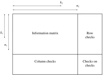
two-dimensional code with an (n1;k1;d1) vertical code, C1, and an (n2;k2;d2) horizontal

code, C2. The resulting code, C, is an (n1n2;k1k2;d1d2) code (Figure 2.1). The term

product code is sometimes applied to array codes; the two terms are interchangeable.

General Properties of Array Codes

Theorem 2.1 The minimum weight for the product of two codes is the product of the

minimum weights of the codes.

Proof 2.1 [Elias, 1954]. The minimum weights of the component codes,C1andC2are

(35)

2.1. BLOCK CODES 13

k1

k2

n1

n2

Information matrix Row

checks

[image:35.595.130.489.129.392.2]

Column checks Checks on

Figure 2.1: Array code.

elements, and each row containing a non-zero element must have at least d2non-zero

elements. Therefore if the product code C contains any non-zero elements it must

contain at least d1 non-zero rows and d2non-zero columns. The minimum number of

non-zero elements is therefore d1d2 and thus the minimum weight ofC is d1d2.

Encoding and decoding are greatly simplified when the component codes are

sys-tematic. For a two-dimensional product code with systematic component codes the

generator matrix can be shown to be the Kronecker product (denoted by ) of the

generator matrices [Slepian, 1960]. For the case when the component codes are single

parity-check codes (i.e., k1 = n1 1, k2 = n2 1) the generator matrix reduces to

(36)

2.1. BLOCK CODES 14

dimensions are possible. As both row and column codes are linear it is not important

whether the row or column encoding is performed first, the checks-on-checks will be

identical in either case [Peterson and Weldon, 1972, p. 132]. Similarly, the decoding

order is not important.

If serial transmission of the codeword symbols is assumed (which is the normal

case) the two-dimensional codeword, v

v= 2 6 6 6 6 6 6 6 6 6 4

v0;0 v0;1

::: v0 ;n2 1

v1;0 v1;1

::: v1 ;n2 1

..

. ... . .. ...

vn1 1;0 vn1 1;1

::: vn

1 1;n2 1 3 7 7 7 7 7 7 7 7 7 5 (2.10)

must be converted to a one-dimensional vector before transmission over the channel.

The mapping of vi;j where 0

i < n1 and 0 j < k2 to vl where 0 l < n1n2 1

may be accomplished by a number of methods. The canonical ordering is achieved

by choosing i and j as the quotient and remainder when l is divided by n2[Berlekamp,

1968, p. 338]. Canonical ordering gives the array

v= 2 6 6 6 6 6 6 6 6 6 4

v0 v1 ::: vn

2 1

vn2 vn2+1

::: v2n

2 1

..

. ... . .. ...

v(n1 1)n2 v(n1 1)n2+1

::: vn 1 3 7 7 7 7 7 7 7 7 7 5 (2.11)

For the case when n1 and n2 are relatively prime there is (by the Chinese remainder

(37)

2.1. BLOCK CODES 15

l i mod n2 and l j mod n1 [Burton and Weldon, 1965]. This mapping of i and j

to l is known as cyclic ordering. The reasoning behind the name is clearly seen from

the example below where n1 =3 and n2 =5

v= 2

6 6 6 6 6 4

v0 v6 v12 v3 v9

v10 v1 v7 v13 v4

v5 v11 v2 v8 v14

3

7 7 7 7 7 5

(2.12)

If C1 andC2 are cyclic codes and n1 and n2 are relatively prime then the product

C =C1C2 is also cyclic, however not all cyclic codes are array codes [MacWilliams

and Sloane, 1978, p. 570].

Decoding Array Codes

Many decoding algorithms for array codes exist, both algebraic and trellis-oriented.

The simplest method for decoding a canonically-ordered array code is to cascade

de-code the component de-codes one at a time, decoding the row de-code,C2, and then the

col-umn codeC1. Particularly for memoryless channels, the cascade decoding algorithm

is inefficient. There exist error patterns for which the code is capable of correcting but

the algorithm fails to correct. If the minimum distances, d1 and d2, of the component

codes are odd then there are error patterns of weight (d1 +1)(d2 +1)=4 which are

incorrectly decoded, although the code is capable of correcting errors up to weight

(38)

2.1. BLOCK CODES 16

2.1.5 Generalised Array Codes

As the name suggests GACs are a generalisation of the array codes introduced by

Elias. Unlike standard array codes GACs may have different component codes along

a given dimension, with the restriction of the code length being invariant. The total

number of code symbols is given by n = n1n2, where n1 and n2 are the number of

rows and columns, respectively. The total number of information symbols is given by

k= P

n1

i=1

kp, where kp is the number of information symbols in p-th row [Honary and

Markarian, 1997, p. 11].

The technique provides a simple design procedure for constructing many

differ-ent block codes, BCH, Hamming, Golay, RM etc. [Honary and Markarian, 1993a,b;

Honary et al., 1995a]. It is important as it allows minimal trellises to be designed in a

straightforward manner.

2.1.6 Cyclic codes

Cyclic codes are an important subclass of linear block codes, not only because many

prominent codes are cyclic e.g., BCH, RS, but also because they are used in the

con-struction of other error-correcting codes e.g., Kerdock and Preparata codes. The

inher-ent algebraic structure of cyclic codes allows the formation of many practical

decod-ing methods; Euclidean (Section 3.3), Berlekamp-Massey (Section 3.4), step-by-step

(39)

2.1. BLOCK CODES 17

General Properties of Cyclic Codes

A code C is cyclic if it is linear and every cyclic shift of every codeword v is also a

codeword. i.e., if (v0; v1; :::; vn 1) is a codeword in C then (vn 1; v0; :::; vn 2)

is also a codeword in C [MacWilliams and Sloane, 1978, p. 188]. Cyclic codes are

commonly defined in terms of polynomials, where the coefficients of the polynomial

are the symbols in v. The notation v(x) will be used to denote a code polynomial. The

relationship between a codeword v and the polynomial is

v=(v0; v1; :::; vn 1) (2.13)

v(x)=v0+v1x+v2x

2

+:::+vn 1x

n 1

(2.14)

It can be seen that the maximum degree of v(x) is n 1. Algebraically, v(x) is defined

to be a polynomial modulo Xn _{1. This leads to the important identity}

xn

1 (2.15)

From (2.15) it can be shown that a multiplication of v(x) by x is a cyclic shift

x:v(x)=

=

v0x+v1x

2

+v2x

3

+::: +vn 2x

n 1

+vn 1x

n

vn 1+v0x+v1x

2

+v2x

3

+::: +vn 2x

n 1

(2.16)

It can be shown [Wicker, 1994, p. 101; Wilson, 1996, pp. 443–444] that there

(40)

2.1. BLOCK CODES 18

a product of the generator polynomial

v(x)=u(x) g(x) (2.17)

where u(x) is a polynomial of degree k 1 or less and is known as the message

polynomial. Equation (2.17) indicates a method by which a message polynomial, u(x),

can be encoded to its corresponding codeword polynomial. An alternative approach

is based on matrices. It is shown in equation (2.2) that a generator matrix can be

constructed from k linearly independent codewords. Since the generator polynomial

is itself a codeword polynomial (corresponding to the case u(x)=1) the k codewords

can be arranged as k cyclic shifts of g(x).

G= 2 6 6 6 6 6 6 6 6 6 6 6 6 4 g(x) xg(x) x2_g(x)

.. .

xk 1

g(x) 3 7 7 7 7 7 7 7 7 7 7 7 7 5 = 2 6 6 6 6 6 6 6 6 6 6 6 6 4

g0 g1 ::: gr 0 ::: 0 0

0 g0 g1 ::: gr 0 ::: 0

. .. ... . ..

0 ::: 0 g0 g1 ::: gr 0

0 0 ::: 0 g0 g1 ::: gr

3 7 7 7 7 7 7 7 7 7 7 7 7 5 (2.18)

The encoding procedure given in (2.17) does not produce a systematic codeword.

Normally, systematic codewords are preferred as they simplify the decoding

proce-dure. The normal method by which systematic codewords are generated is [Michelson

and Levesque, 1985, p. 133]

v(x)=

xn k

u(x) mod g(x)

+x

n k

(41)

2.1. BLOCK CODES 19

It can be seen that this does result in a valid codeword, the remainder when v(x) is

divided by g(x) is zero, and the maximum degree of v(x) is n 1.

Syndrome Polynomial

For cyclic codes (e.g., BCH and RS) the calculation of the syndromes can be

per-formed more efficiently by using the cyclic properties of the code. Though the

syn-drome vector can be calculated by S = rH

T _{(2.7) this calculation can also be}

per-formed as

S(x)=

r(x) g(x)

=r(x) mod g(x)

(2.20)

where S(x)=S1+S2x+S3x

2

+:::+S2tx

2t 1

(2.21)

where S(x) is the syndrome polynomial. Thus the syndrome polynomial may be

de-fined as the remainder when an erroneous codeword is divided by the generator

poly-nomial, g(x). The proof is given in [Peterson and Weldon, 1972, p. 231]. For the

case of the received codeword being equal to the transmitted codeword, v(x), the

syn-drome polynomial is zero since valid codewords are exactly divisible by the generator

polynomial (2.17).

It can be shown that the syndrome polynomial is dependent upon the error

(42)

2.1. BLOCK CODES 20

into (2.20)

S(x)=r(x) mod g(x)

=[v(x)+e(x)℄mod g(x)

=v(x) mod g(x)+e(x) mod g(x)

=e(x) mod g(x)

(2.22)

since v(x) mod g(x)=0 (from (2.17)).

2.1.7 Bose-Chaudhuri-Hocquenghem Codes

Bose-Chaudhuri-Hocquenghem codes were discovered independently by

Hocqueng-hem [HocquengHocqueng-hem, 1959] in 1959 and Bose and Chaudhuri [Bose and

Ray-Chaudhuri, 1960a,b] in 1960. BCH codes are a generalisation of the cyclic Hamming

codes for correcting multiple errors. Peterson [Peterson, 1960] proved that BCH codes

are cyclic. Gorenstein and Zierler [Gorenstein and Zierler, 1961] generalised the BCH

codes for non-binary alphabets of size pm_{. Their wide choice of block lengths, code}

rates and symbol alphabets, coupled with efficient decoding algorithms, has made

BCH codes a popular choice for many communication systems.

General Properties of BCH Codes

When constructing an arbitrary cyclic code there is no guarantee of the minimum

distance of the code produced [Wicker, 1994, p. 176]. It is necessary to conduct a

(43)

2.1. BLOCK CODES 21

and thus the minimum distance of the code. For BCH codes this procedure is not

required, the BCH bound places lower limit on the minimum distance of the code. An

understanding of these codes requires a knowledge of finite field arithmetic [McEliece,

1987].

Theorem 2.2 The BCH Bound [Wicker, 1994]

Let C be a q-ary (n;k) cyclic code with generator polynomial g(x). Let m be the

multiplicative order of q mod n. (GF(qm_{) is thus the smallest extension field of GF(q)}

which contains a primitive n-th root of unity.) Let be a primitive n-th root of unity.

Select g(x) to be a minimal-degree polynomial in GF(q)[x℄, where GF(q)[x℄

de-notes the collection of all polynomials a0+a1x+a2x

2

++x

n _{of arbitrary degree}

with coefficientsfaigin the finite field GF(q) [Wicker, 1994, p. 40], such that

g(

b

)=g(

b+1

)=g(

b+2

)==g(

b+Æ 2

)=0 (2.23)

for some integers b 0 and Æ 1. The roots of the generator polynomial g(x) are

Æ 1 consecutive powers of . The codeC defined by g(x) has minimum distance

d Æ.

Proof of Theorem 2.2 can be found in [MacWilliams and Sloane, 1978; Peterson and

Weldon, 1972; Wicker, 1994]. The BCH bound can be used to produce a BCH code

with a given design distance. However, since the weight distributions of most BCH

codes are not known the actual minimum distance may be greater than the design

(44)

2.1. BLOCK CODES 22

Generator Polynomial

The generator polynomial for a BCH code has 2t roots, which are consecutive powers

of (from Theorem 2.2). Therefore

g(x)=

2t 1

Y

i=0

(x

b+i

) (2.24)

For the case when b=1 the code is termed narrow sense [MacWilliams and Sloane,

1978, p. 203].

2.1.8 Reed-Solomon Codes

Reed-Solomon codes were discovered by Reed and Solomon in 1960 and are a

spe-cial subclass of non-binary BCH codes [Reed and Solomon, 1960]. RS codes exhibit

additional properties to BCH codes which make them very much more powerful than

BCH codes. Their powerful error-correcting abilities have made them possibly the

most important codes. RS codes are multi-level, therefore log₂q binary bits are

com-monly mapped to one RS symbol. This process provides some burst-error correction.

They have many and widespread applications which include the compact disc, satellite

communications and digital video broadcasting.

General Properties of RS Codes

Reed-Solomon codes are cyclic and so profit from the many useful characteristics

cyclic codes offer. They are normally generated in systematic form using (2.19).

(45)

2.1. BLOCK CODES 23

Proof 2.2 LetC be an (n;k) RS code. The Singleton bound (Section 2.1.3) gives an

upper bound of d n k+1 to all (n;k) codes. The BCH bound provides a lower

bound. The generator polynomial g(x) is of degree n k, so it contains n k =

Æ 1 consecutive powers of a primitive n-th root of unity. Therefore d n k+1.

Combining these two results gives

d =n k+1 (2.25)

Theorem 2.3 and its proof are important for two reasons. Firstly it shows that RS

codes can be designed such that their designed minimum distance is always the actual

minimum distance (unlike BCH codes). Secondly, RS codes satisfy the Singleton

bound with equality, so they are maximum distance separable.

Theorem 2.4 RS codes are invertible.

A code is said to be invertible if any k symbols can be used as information symbols

in a systematic representation. This follows from the MDS property, proof is given

(46)

2.2. CONVOLUTIONAL CODES 24

2.2 Convolutional Codes

2.2.1 Overview

The name convolutional code was coined by Elias [Elias, 1955] to describe a code

which is the output sequence of a linear mapping of an input sequence with a

discrete-time, finite-alphabet convolution of the input and encoder’s impulse response [Wilson,

1996, p. 551]. Such codes are sometimes termed trellis codes, but this name is

mis-leading because block codes may also be represented by trellises. The concept of

encoding an input sequence without segmenting it is very different to that used by

block codes (Section 2.1).

Input bit

First code symbol

Output branch word

Second code symbol

Figure 2.2: Encoder for (2;1;3) convolutional code.

2.2.2 General Properties

A convolutional code over GF(q) is usually described by the parameters (n;k;K),

where k is the number of q-ary symbols (simultaneously) input to the decoder and n

(47)

2.3. CONCATENATED CODES 25

block code, the rate is given by n=k. The constraint length of the code, K, is defined as

the number of consecutive symbols in the output stream affected by any input symbol.

It is also the memory of the code.

2.3 Concatenated Codes

2.3.1 Overview

Concatenated coding was introduced in 1966 by Forney [Forney, 1966]. It is a

pow-erful technique for creating error-correcting codes by combining two (or more) codes

sequentially. The primary reason for using concatenated codes is to achieve a low

error rate with an overall implementation complexity which is less than that which

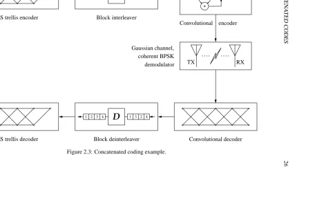
would be required by a single decoding operation [Sklar, 1988, p. 365]. Figure 2.3

shows a concatenated coding scheme. The data stream is first encoded with the outer

code (in this case an RS block code). The output of the outer code is then re-encoded

with the inner code, (here a convolutional code) before transmission. At the receiver

the decoding order must be reversed, and so the inner code is decoded first. Any errors

from the output of the inner decoder are likely to appear as bursts, hence it is usual

to include an interleaver and de-interleaver between the inner and outer codes. The

purpose of the interleaver is to rearrange the symbols so that errors do not occur in

bursts but are spread through several outer codewords to allow correct decoding.

Convolutional codes are a natural choice for the inner code. With a suitable

Vit-erbi decoder SD information can be used for maximum performance. RS codes are

(48)

2

.3

.

C

O

N

C

A

T

E

N

A

T

E

D

C

O

D

E

S

2

6

1 2 3 4

I

1 3 2 4

1 2 3 4

D

1 3 2 4

RS trellis encoder Block interleaver

Convolutional encoder

Gaussian channel, coherent BPSK demodulator

RS trellis decoder Block deinterleaver Convolutional decoder

[image:48.595.126.717.123.461.2]

TX RX

(49)

2.4. TRELLISES 27

binary convolutional code the burst-error performance of the RS code helps minimise

errors. There are, however, many possible configurations for a concatenated coding

scheme and flexibility is one of its many advantages. For example the compact disc

coding system uses a concatenated system based upon RS(32;28;5) and RS(28;24;5)

shortened RS codes.

2.3.2 General Properties of Concatenated Codes

The rate of a concatenated code is the product of the rates of its component codes.

Consider a concatenated codeC with an (n1;k1;d1) inner code C1 and an (n2;k2;d2)

outer codeC2. An input sequence of k1k2symbols is passed to the outer encoder. The

output is k1n2 symbols. This new block is sent to the inner decoder which results in

n1n2output symbols. The rate is thus

k1k2

n1n2.

The minimum distance of a concatenated code is d1d2 [Lin and Costello, 1983,

p. 279].

The proof is the same as for an array code, see Proof 2.1.

2.4 Trellises

2.4.1 Introduction

A trellis diagram (commonly called a trellis) is an acyclic edge-labelled directed

graph [Muder, 1988], with one start point (the root) and one end point (the goal).

(50)

2.4. TRELLISES 28

be viewed as a two-dimensional representation of the qk _{codewords through the}

n-dimensional codespace. To enable an accurate description of the properties of a trellis

it is first necessary to introduce some common definitions.

2.4.2 Definitions

Nodes of the graph represent possible encoder states, Si;t, where i is the state number

and t is the time index. The nodes are decomposed into a union of disjoint subsets,

called vertices or levels. The levels are numerated 0; 1; ::: ; Nc(Nc n+1) and the

t-th level consists of Nt nodes, (S1;t) ; (S2

;t)

; ::: ; (SN

t;t).

Between states in adjacent levels, Si;t and Sj;t+1, there may be directed branches

(also called edges), B(Si;t !Sj

;t+1), which indicate possible changes in state. Branches

are only permitted to connect adjacent levels. The set of branches between level t 1

and t is called the t-th depth. In some texts the set of branches at a given depth is

termed a stage [Wicker, 1994, p. 292]. To prevent confusion (e.g., with “two-stage

decoding”) such terminology is avoided in this work. Associated with every branch is

a label denoting the output (or code) symbol(s) given when that branch is taken, and

a branch metric, Bm, which indicates the likelihood of a given branch being selected.

For certain trellises an additional input (or data) label may exist. Its purpose is to allow

the same trellis structure to be used for both encoding and decoding operations. The

code label is a lt-dimensional vector of q-ary symbols, (l1; l2; :::; lt). The code label

associated with the branch B(Si;t !Sj

;t+1) is denoted by L(Si;t ;Sj

;t+1).

Using the notation introduced above the root can be more precisely defined as S1;0,

(51)

2.4. TRELLISES 29

by P(Si ;t

! Sj ;t+1

! Sk ;t+2

! ::: ! Sz

;t+Æ). The term partial path is sometimes

used to denote a sequence of branches for which decoding is incomplete, thus the

sequence starts from the root but does not reach the goal. For certain codes (generally

convolutional codes) it is necessary to truncate the trellis to lessen decoding delay.

Frequently these trellises are shown with multiple roots and goals (see Figure 4.7

for an example). Though this does not strictly match the definition of a trellis, the

truncated section is often considered to be a trellis in its own right.

A trellis is called a code trellis of the code C if there is a one-to-one mapping

between the codewords of the code C and all paths between S1

;0 and S1;Nc (i.e., all P(S1

;0

!:::!S1 ;Nc)).

LetN(t ) =[N0; N1; :::; NN

c℄be the state profile of the trellis T andB(t ) =[B1;

B2; ::: ; BN

c℄be the branch profile, whereNi is the number of states at the i-th level

andBj is the number of branches at the j-th depth [Forney and Trott, 1993; Honary

and Markarian, 1997, p. 161]. LetL(t ) = [L1; L2; :::; LN

c℄be the label size profile

of the trellis whereLj is the number of symbols used for labelling the j-th depth.

Figure 2.4 shows a trellis for the (7;4;3) Hamming code annotated with the

(52)

2

.4

.

T

R

E

L

IS

E

S

3

0

branch label path (bold)

goal root

branch

state

level:

depth:

0

1

2

3

4 4 00=00

10

=

11

01

=

01

1₁

=

1₀

0=00

1=11

0=01 0=01

0=01

1=10

=00

=

11

=

01

=

10

(53)

2.4. TRELLISES 31

this trellis are

N(t )=[N0;N1;N2;N3;N4℄

=[1;4;4;4;1℄

(2.26)

B(t )=[B1;B2;B3;B4℄

=[4;8;8;4℄

(2.27)

L(t )=[L1;L2;L3;L4℄

=[2;2;2;1℄

(2.28)

2.4.3 Properties

Proper A trellis where all the branches (edges) leaving any state (vertex) have distinct

labels. Unless otherwise stated all references to a trellis will imply a proper

trellis.

Observable A trellis with a one-to-one mapping between all codewords of the codeC

and all paths between S1;0 and S1;Nc (i.e., all P(S1

;0

!:::!S1 ;Nc)).

Since an unobservable trellis contains more than one path through the trellis

for at least one codeword this may cause difficulties for encoders and for

sub-optimum decoders operating with a reduced-search Viterbi algorithm, or similar

methods.

Minimal trellis Many definitions of a minimal trellis exist due to varying

(54)

2.5. CHANNEL MODELS 32

Muder [Muder, 1988]. The trellis T is a minimal trellis of the codeCif for every

other trellis T0

ofC,Ni N 0

i [Honary and Markarian, 1997, p. 61].

State-Oriented form The trellis state number is directly correlated with the encoder

state.

2.5 Channel Models

2.5.1 Discrete Memoryless Channel

A discrete memoryless channel features discrete input and output alphabets. The set

of conditional probabilities relating the output to the input is given by p( jji) where i

(1 i M) is a modulator M-ary input symbol and j (1 j q) is a demodulator

q-ary output symbol. Thus p( jji) is the probability of receiving j if i was transmitted.

The output symbol depends only on the input symbol, not on the existencre of any

previous errors (hence the channel has no memory). For an input sequence U = u1;

u2; ::: ; uN the conditional probability of the output sequence Z = z1; z2; :::; zN

is [Sklar, 1988, p. 261]

p(ZjU)=

N

Y

m=1

(55)

2.5.2 Binary Symmetric Channel

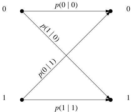
A binary symmetric channel is a special case of the discrete memoryless channel. The

input alphabet size is 2, containing the binary elements “0” and “1”. In addition, the

conditional probabilities are symmetric:

p(0j1) = p(1j0) = p (2.30)

p(0j0) = p(1j1) =1 p (2.31)

The channel transition probabilities (2.30, 2.31) give the probability that a

trans-mitted symbol is received incorrectly. The demodulator makes no attempt to indicate

how well a symbol is received, it merely outputs a “0” or “1”. This type of output is

termed hard decision.

p(0j0)

p(0

j

1)

p(1 j

0)

p(1j1)

0 0

[image:55.595.204.415.456.635.2]

1 1

Figure 2.5: Binary symmetric channel model.

(56)

error-2.5. CHANNEL MODELS 34

correcting code operating over a BSC can be obtained by considering the probability

that>t symbol errors occur [Lin and Costello, 1983]

PM

n

X

i=t+1

n i

Ps i

(1 Ps) n i

(2.32)

2.5.3 Binary Symmetric Erasure Channel

The binary symmetric erasure channel may be viewed as a special case of the DMC,

or as an extension of the BSC. Like the BSC the input alphabet size is 2, containing

the binary elements. However the output alphabet size is increased to 3, and contains

“0”, “1” and an erasure (denoted by “?”). For times when the demodulator is not able

to clearly identify a “0” or “1” it may signal its uncertainty by outputting an erasure.

The decoder is then aware that the symbol is unreliable. The symmetric conditional

probabilities are

p(0j1)= p(1j0)= p (2.33)

p(0j?)= p(1j?)=q (2.34)

(57)

p(0j0)

p(0 j?)

p(0 j

0)

p(1

j

0)

p(1j?)

p(1j1)

0 0

1 1

?

Figure 2.6: Binary symmetric erasure channel model.

2.5.4 Additive White Gaussian Noise Channel

In many cases channels are not discrete but feature a continuous output alphabet over

the range ( 1!+1). An AWGN channel is an example of such a case. The output

is the input with broadband Gaussian noise added. The channel contains no memory

(as defined in Section 2.5.1). This type of channel is an accurate channel model of

many communication systems, such as satellite, deep-space and line-of-sight links.

White Gaussian noise is a random process, with a zero mean and a Gaussian PDF

with variance

2_{. The power spectral density is flat over all frequencies (}

1 f

+1). The channel corrupts the transmitted signal with noise. The probability density

function, y, of the noise value, x, is Gaussian and in the frequency domain the noise is

wideband (or white).

y=

1

p

2

exp

(

1 2

x

2

)

(58)

2.5.5 Quantised AWGN Channel

While channels with continuous output alphabets are a natural phenomenon they are

impossible to use with SD decoding (due to requiring infinite precision to store the

soft value). AWGN channels are frequently ‘approximated’ to a channel with a fixed

number of noise values. Such a channel is termed a quantised additive white Gaussian

noise channel. Like the standard AWGN channel it contains no memory. The

quan-tised AWGN channel is discussed further in Section 5.1.2, where the relative merits

(or metrics) of each quantisation level are calculated and their variation with Eb=N0for

(59)

Chapter 3 Algebraic Decoding of Reed-Solomon

Codes

(60)

Chapter 3 Algebraic Decoding of Reed-Solomon

Codes

3.1 Introduction

While RS codes are constructed by a few well-defined methods (Section 2.1.8) a large

variety of decoding methods have been proposed. An important distinction is between

those which are algebraic and those which are combinatorial in origin. Algebraic

de-coders attempt to correct errors and/or erasures by (algebraically) solving an equation

to find the lowest weight error word. The fundamental method by which most RS

al-gebraic decoders operate is by attempting to solve the key equation. However, not all

algorithms use this approach, notable exceptions being Peterson’s direct method

[Pe-terson, 1960] and Massey’s step-by-step algorithm [Massey, 1965]. In contrast to

algebraic decoders, combinatorial decoders operate on more probabilistic methods to

(61)

3.1. INTRODUCTION 39

find the codeword which most closely matches the received word. Whilst many

alge-braic decoders can be adapted for error-and-erasures decoding it is true to say that they

are unable to make maximum use of soft-decision information in the way that

combi-natorial decoders can. Most combicombi-natorial decoding algorithms are trellis-based (e.g.,

the Fano algorithm and the Viterbi algorithm). Combinatorial decoders are discussed

in Chapter 4.

Some important algebraic decoding algorithms include Euclidean decoding, based

on Euclid’s algorithm and the Berlekamp-Massey algorithm. In 1967 Berlekamp

in-troduced an iterative method for decoding binary BCH codes [Berlekamp, 1967]. In

Peterson’s method the decoding complexity is proportional to the square of the errors

corrected while for Berlekamp’s algorithm the decoding complexity increases linearly

with the number of errors corrected [Wicker, 1994, p. 211]. Thus Berlekamp’s

al-gorithm is much more suited for decoding long block codes where many errors may

be corrected. In 1969 Massey described a “shift-register” synthesis of the Berlekamp

algorithm [Massey, 1969]. The algorithm is now commonly called the

Berlekamp-Massey algorithm in joint commemoration of their findings. In 1975 Sugiyama et al.

showed how Euclid’s algorithm, for finding the greatest common divisor of two

inte-gers or polynomials, can be used to solve the key equation and decode BCH and RS

codes [Sugiyama et al., 1975].

This Chapter begins with a discussion of the key equation (Section 3.2). The

syn-drome, error-locator and error-evaluator polynomials are defined. A method by which

the error values can be calculated is given, along with its proof. Euclidean decoding

(62)

3.2. THE KEY EQUATION 40

Berlekamp-Massey algorithm. The same decoding example is repeated for the case of

BM decoding. Finally, high-speed step-by-step decoding is shown. Again, the same

decoding example is used to illustrate the algorithm. All the algorithms are described

using the same form of the key equation, and have been generalised for the case when

the BCH sense is not narrow (Section 2.1.7).

3.2 The Key Equation

3.2.1 Syndrome Calculation

Many common algebraic decoding algorithms for parity-check block codes start by

testing if the syndromes (Section 2.1.2) of the received codeword are non-zero (i.e., if

the parity checks fail). If the syndrome vector or polynomial is non-zero the received

codeword is in error and error-correction is begun.

Let the received codeword be represented by the polynomial r(x) = r0 +r1x+

::: +rn 1x

n 1_{. Let the error word corrupting the received word be represented by}

the polynomial e(x) = e0 +e1x+:::+en 1x

n 1_{. The syndrome values}1 _S

j, ( j = 1;

2; ::: ; 2t ) is the value of the received polynomial evaluated at the 2t roots used to

define the RS (or BCH) code [Wilson, 1996, p. 471]. Thus, for a narrow sense BCH

code (b= 1) the j-th syndrome is calculated by substituting

j _{for x in r(x). For the}

(63)

more general case

Sj =r(

j+b 1

)

=

n 1

X

i=0

(ri)(

j+b 1

)i

=

n 1

X

i=0

(vi+ei)(

j+b 1

)i

=

n 1

X

i=0

(ei)

i( j+b 1)

where j=1; 2; ::: ; 2t

(3.1)

3.2.2 Error-locator Polynomial

Let the received codeword contain ( t ) correctable errors. Let the locations of

the errors be given by time indices i1; i2; :::; i

. For each symbol in error define an

error-locator, Xisuch that

Xi=

i

(3.2)

Noting that only symbols received in error contribute to the syndrome values it is

possible to rewrite (3.1) in terms of the error-locators

Sj = X

l=1

eilX ( j+b 1)

l (3.3)

The error-locator polynomial,(x), is defined as a polynomial whose inverse roots

(64)

the roots of(x).

(x) 4 =

Y

i=1

(1 Xix) (3.4)

From (3.4) it can be seen that deg(x) = , and that for no errors ( = 0) then

(x) = 0. For binary codes it is sufficient to find the location of an error, since the

error value is always 1. However for RS and other multi-level codes it is necessary

to find the value of each error in addition to the location of each error. It is therefore

necessary to define an additional polynomial to find the value of the error(s).

3.2.3 Error-evaluator Polynomial

The error-evaluator polynomial is a polynomial which when evaluated at an error

lo-cation gives the value of the error. It is defined as follows.2 _{The syndrome polynomial}

is an infinite degree polynomial, however only the first 2t coefficients of x are known

1+S(x)=1+

1 X

j=1

Sjx j

=1+ 1 X

j=1 X

l=1

eilX ( j+b 1)

l

!

xj

=1+ X

l=1

eil

1 X

j=1

X( j+b 1)

l x

j

(3.5)

The summation

P 1

j=1

X( j+b 1)

l x

j _{can be simplified to a rational expression by noting it}

is a geometric series of the form a+ar

1

+ar

2

+:::, for which the simplified form is

2_{This is similar to [Wicker, 1994, p. 221], but has been generalised for the case when b}

Improved error control techniques for data transmission